Photometry with XGA
This tutorial will show you how to generate photometric products (ie. images, exposure maps, and ratemaps) from XGA sources, and cover the basics of interacting with the XGA photometric products, including using source masks and the built in peak finding techniques.
In order to generate these products, XGA must interact with telescope-specific software, such as SAS for XMM and eSASS for eROSITA, therefore the user must have the appropriate software installed to interact with certain data. XGA will check for the presence of the relevant software before trying to run any routines that depend on it.
This demonstration will detail the XGA features that are common to every supported telescope. However, please note that products made from different telescopes will have certain telescope-specific quirks associated with them, that arise from interaction with their corresponding software - e.g. the way XMM’s SAS generates images is different to the way eROSITA’s eSASS does. Consequently, there will be some differing optional arguments available within XGA’s built in functions that interact with these softwares. It is therefore important to readthe multi mission tutorial, where caveats associated with interacting with telescope-specific software are detailed, along with reccomendations, and useful tips when considering data from certain telescopes.
[1]:
from astropy.units import Quantity
from astropy.visualization import LinearStretch
import numpy as np
import pandas as pd

from xga.sources import GalaxyCluster, NullSource
from xga.samples import ClusterSample
from xga.generate.sas import evselect_image, eexpmap, emosaic
from xga.generate.esass import evtool_image, expmap
from xga.utils import xmm_sky
/mnt/lustre/projects/astro/general/jp735/XGA_dev/XGA/xga/utils.py:39: DeprecationWarning: The XGA 'find_all_wcs' function should be imported from imagetools.misc, in the future it will be removed from utils.
  warn(message, DeprecationWarning)
/its/home/jp735/.conda/envs/xga_dev/lib/python3.8/site-packages/regions/_geometry/__init__.py:8: DeprecationWarning: `np.bool` is a deprecated alias for the builtin `bool`. To silence this warning, use `bool` by itself. Doing this will not modify any behavior and is safe. If you specifically wanted the numpy scalar type, use `np.bool_` here.
Deprecated in NumPy 1.20; for more details and guidance: https://numpy.org/devdocs/release/1.20.0-notes.html#deprecations
  from .polygonal_overlap import *
First we declare both an individual galaxy cluster source object, and a galaxy cluster sample object; in order to show that the generation of products from individual sources and samples of sources is done in the same way. The sample of four clusters is taken from the DES-Y1 sample (Farahi et al. 2019), and the individual cluster is Abell 907.
[2]:
# Setting up the column names and numpy array that go into the Pandas dataframe
column_names = ['name', 'ra', 'dec', 'z', 'r500', 'richness', 'richness_err']
cluster_data = np.array([['DEMO-1', 40.912, -48.561, 0.495, 2.539, 138.504, 4.243],
                         ['DEMO-2', 41.353, -53.029, 0.300, 4.720, 150.571, 4.141],
                         ['DEMO-3', 43.565, -58.953, 0.428, 3.292, 221.674, 5.713],
                         ['DEMO-4', 79.156, -54.500, 0.299, 3.870, 207.243, 7.181]])

sample_df = pd.DataFrame(data=cluster_data, columns=column_names)
sample_df[['ra', 'dec', 'z', 'r500', 'richness', 'richness_err']] = \
    sample_df[['ra', 'dec', 'z', 'r500', 'richness', 'richness_err']].astype(float)

# Defining the sample of four DES galaxy clusters
demo_smp = ClusterSample(sample_df["ra"].values, sample_df["dec"].values, sample_df["z"].values,
                         sample_df["name"].values,
                         r500=Quantity(sample_df["r500"].values, 'arcmin'),
                         richness=sample_df['richness'].values,
                         richness_err=sample_df['richness_err'].values,
                         search_distance={'erosita': Quantity(2, 'deg')})

# And defining an individual source object for Abell 907
demo_src = GalaxyCluster(149.59209, -11.05972, 0.16, r500=Quantity(1200, 'kpc'), r200=Quantity(1700, 'kpc'),
                         name="A907", search_distance={'erosita': Quantity(3, 'deg'),
                                     'xmm': Quantity(30, 'arcmin')})
/its/home/jp735/.conda/envs/xga_dev/lib/python3.8/site-packages/ipykernel/ipkernel.py:283: DeprecationWarning: `should_run_async` will not call `transform_cell` automatically in the future. Please pass the result to `transformed_cell` argument and any exception that happen during thetransform in `preprocessing_exc_tuple` in IPython 7.17 and above.
  and should_run_async(code)
Declaring BaseSource Sample:   0%|          | 0/4 [00:00<?, ?it/s]/mnt/lustre/projects/astro/general/jp735/XGA_dev/XGA/xga/sources/base.py:188: UserWarning: A dictionary of search distances that did not contain all requested telescopes has been passed, default values have been used for the missing telescopes.
  matches, excluded = separation_match(ra, dec, search_distance, telescope)
Declaring BaseSource Sample:  25%|██▌       | 1/4 [00:00<00:00,  6.36it/s]/mnt/lustre/projects/astro/general/jp735/XGA_dev/XGA/xga/sources/base.py:188: UserWarning: A dictionary of search distances that did not contain all requested telescopes has been passed, default values have been used for the missing telescopes.
  matches, excluded = separation_match(ra, dec, search_distance, telescope)
Declaring BaseSource Sample:  50%|█████     | 2/4 [00:00<00:00,  6.19it/s]/mnt/lustre/projects/astro/general/jp735/XGA_dev/XGA/xga/sources/base.py:188: UserWarning: A dictionary of search distances that did not contain all requested telescopes has been passed, default values have been used for the missing telescopes.
  matches, excluded = separation_match(ra, dec, search_distance, telescope)
Declaring BaseSource Sample:  75%|███████▌  | 3/4 [00:00<00:00,  6.52it/s]/mnt/lustre/projects/astro/general/jp735/XGA_dev/XGA/xga/sources/base.py:188: UserWarning: A dictionary of search distances that did not contain all requested telescopes has been passed, default values have been used for the missing telescopes.
  matches, excluded = separation_match(ra, dec, search_distance, telescope)
Declaring BaseSource Sample: 100%|██████████| 4/4 [00:00<00:00,  5.97it/s]
Generating products of type(s) ccf: 100%|██████████| 8/8 [00:15<00:00,  1.91s/it]
Generating products of type(s) image: 100%|██████████| 4/4 [00:00<00:00,  8.17it/s]
Generating products of type(s) expmap: 100%|██████████| 4/4 [00:00<00:00,  8.98it/s]
Setting up Galaxy Clusters:   0%|          | 0/4 [00:00<?, ?it/s]/mnt/lustre/projects/astro/general/jp735/XGA_dev/XGA/xga/sources/base.py:188: UserWarning: A dictionary of search distances that did not contain all requested telescopes has been passed, default values have been used for the missing telescopes.
  matches, excluded = separation_match(ra, dec, search_distance, telescope)
/its/home/jp735/.conda/envs/xga_dev/lib/python3.8/site-packages/regions/core/compound.py:93: DeprecationWarning: `np.int` is a deprecated alias for the builtin `int`. To silence this warning, use `int` by itself. Doing this will not modify any behavior and is safe. When replacing `np.int`, you may wish to use e.g. `np.int64` or `np.int32` to specify the precision. If you wish to review your current use, check the release note link for additional information.
Deprecated in NumPy 1.20; for more details and guidance: https://numpy.org/devdocs/release/1.20.0-notes.html#deprecations
  data = self.operator(*np.array(padded_data, dtype=np.int))
Setting up Galaxy Clusters:  25%|██▌       | 1/4 [00:10<00:31, 10.61s/it]/mnt/lustre/projects/astro/general/jp735/XGA_dev/XGA/xga/sources/base.py:188: UserWarning: A dictionary of search distances that did not contain all requested telescopes has been passed, default values have been used for the missing telescopes.
  matches, excluded = separation_match(ra, dec, search_distance, telescope)
/its/home/jp735/.conda/envs/xga_dev/lib/python3.8/site-packages/regions/core/compound.py:93: DeprecationWarning: `np.int` is a deprecated alias for the builtin `int`. To silence this warning, use `int` by itself. Doing this will not modify any behavior and is safe. When replacing `np.int`, you may wish to use e.g. `np.int64` or `np.int32` to specify the precision. If you wish to review your current use, check the release note link for additional information.
Deprecated in NumPy 1.20; for more details and guidance: https://numpy.org/devdocs/release/1.20.0-notes.html#deprecations
  data = self.operator(*np.array(padded_data, dtype=np.int))
/its/home/jp735/.conda/envs/xga_dev/lib/python3.8/site-packages/regions/core/compound.py:93: DeprecationWarning: `np.int` is a deprecated alias for the builtin `int`. To silence this warning, use `int` by itself. Doing this will not modify any behavior and is safe. When replacing `np.int`, you may wish to use e.g. `np.int64` or `np.int32` to specify the precision. If you wish to review your current use, check the release note link for additional information.
Deprecated in NumPy 1.20; for more details and guidance: https://numpy.org/devdocs/release/1.20.0-notes.html#deprecations
  data = self.operator(*np.array(padded_data, dtype=np.int))
/its/home/jp735/.conda/envs/xga_dev/lib/python3.8/site-packages/regions/core/compound.py:93: DeprecationWarning: `np.int` is a deprecated alias for the builtin `int`. To silence this warning, use `int` by itself. Doing this will not modify any behavior and is safe. When replacing `np.int`, you may wish to use e.g. `np.int64` or `np.int32` to specify the precision. If you wish to review your current use, check the release note link for additional information.
Deprecated in NumPy 1.20; for more details and guidance: https://numpy.org/devdocs/release/1.20.0-notes.html#deprecations
  data = self.operator(*np.array(padded_data, dtype=np.int))
/its/home/jp735/.conda/envs/xga_dev/lib/python3.8/site-packages/regions/core/compound.py:93: DeprecationWarning: `np.int` is a deprecated alias for the builtin `int`. To silence this warning, use `int` by itself. Doing this will not modify any behavior and is safe. When replacing `np.int`, you may wish to use e.g. `np.int64` or `np.int32` to specify the precision. If you wish to review your current use, check the release note link for additional information.
Deprecated in NumPy 1.20; for more details and guidance: https://numpy.org/devdocs/release/1.20.0-notes.html#deprecations
  data = self.operator(*np.array(padded_data, dtype=np.int))
/its/home/jp735/.conda/envs/xga_dev/lib/python3.8/site-packages/regions/core/compound.py:93: DeprecationWarning: `np.int` is a deprecated alias for the builtin `int`. To silence this warning, use `int` by itself. Doing this will not modify any behavior and is safe. When replacing `np.int`, you may wish to use e.g. `np.int64` or `np.int32` to specify the precision. If you wish to review your current use, check the release note link for additional information.
Deprecated in NumPy 1.20; for more details and guidance: https://numpy.org/devdocs/release/1.20.0-notes.html#deprecations
  data = self.operator(*np.array(padded_data, dtype=np.int))
/its/home/jp735/.conda/envs/xga_dev/lib/python3.8/site-packages/regions/core/compound.py:93: DeprecationWarning: `np.int` is a deprecated alias for the builtin `int`. To silence this warning, use `int` by itself. Doing this will not modify any behavior and is safe. When replacing `np.int`, you may wish to use e.g. `np.int64` or `np.int32` to specify the precision. If you wish to review your current use, check the release note link for additional information.
Deprecated in NumPy 1.20; for more details and guidance: https://numpy.org/devdocs/release/1.20.0-notes.html#deprecations
  data = self.operator(*np.array(padded_data, dtype=np.int))
Setting up Galaxy Clusters:  50%|█████     | 2/4 [00:22<00:22, 11.29s/it]/mnt/lustre/projects/astro/general/jp735/XGA_dev/XGA/xga/sources/base.py:188: UserWarning: A dictionary of search distances that did not contain all requested telescopes has been passed, default values have been used for the missing telescopes.
  matches, excluded = separation_match(ra, dec, search_distance, telescope)
/its/home/jp735/.conda/envs/xga_dev/lib/python3.8/site-packages/regions/core/compound.py:93: DeprecationWarning: `np.int` is a deprecated alias for the builtin `int`. To silence this warning, use `int` by itself. Doing this will not modify any behavior and is safe. When replacing `np.int`, you may wish to use e.g. `np.int64` or `np.int32` to specify the precision. If you wish to review your current use, check the release note link for additional information.
Deprecated in NumPy 1.20; for more details and guidance: https://numpy.org/devdocs/release/1.20.0-notes.html#deprecations
  data = self.operator(*np.array(padded_data, dtype=np.int))
/its/home/jp735/.conda/envs/xga_dev/lib/python3.8/site-packages/regions/core/compound.py:93: DeprecationWarning: `np.int` is a deprecated alias for the builtin `int`. To silence this warning, use `int` by itself. Doing this will not modify any behavior and is safe. When replacing `np.int`, you may wish to use e.g. `np.int64` or `np.int32` to specify the precision. If you wish to review your current use, check the release note link for additional information.
Deprecated in NumPy 1.20; for more details and guidance: https://numpy.org/devdocs/release/1.20.0-notes.html#deprecations
  data = self.operator(*np.array(padded_data, dtype=np.int))
/its/home/jp735/.conda/envs/xga_dev/lib/python3.8/site-packages/regions/core/compound.py:93: DeprecationWarning: `np.int` is a deprecated alias for the builtin `int`. To silence this warning, use `int` by itself. Doing this will not modify any behavior and is safe. When replacing `np.int`, you may wish to use e.g. `np.int64` or `np.int32` to specify the precision. If you wish to review your current use, check the release note link for additional information.
Deprecated in NumPy 1.20; for more details and guidance: https://numpy.org/devdocs/release/1.20.0-notes.html#deprecations
  data = self.operator(*np.array(padded_data, dtype=np.int))
/its/home/jp735/.conda/envs/xga_dev/lib/python3.8/site-packages/regions/core/compound.py:93: DeprecationWarning: `np.int` is a deprecated alias for the builtin `int`. To silence this warning, use `int` by itself. Doing this will not modify any behavior and is safe. When replacing `np.int`, you may wish to use e.g. `np.int64` or `np.int32` to specify the precision. If you wish to review your current use, check the release note link for additional information.
Deprecated in NumPy 1.20; for more details and guidance: https://numpy.org/devdocs/release/1.20.0-notes.html#deprecations
  data = self.operator(*np.array(padded_data, dtype=np.int))
/its/home/jp735/.conda/envs/xga_dev/lib/python3.8/site-packages/regions/core/compound.py:93: DeprecationWarning: `np.int` is a deprecated alias for the builtin `int`. To silence this warning, use `int` by itself. Doing this will not modify any behavior and is safe. When replacing `np.int`, you may wish to use e.g. `np.int64` or `np.int32` to specify the precision. If you wish to review your current use, check the release note link for additional information.
Deprecated in NumPy 1.20; for more details and guidance: https://numpy.org/devdocs/release/1.20.0-notes.html#deprecations
  data = self.operator(*np.array(padded_data, dtype=np.int))
/its/home/jp735/.conda/envs/xga_dev/lib/python3.8/site-packages/regions/core/compound.py:93: DeprecationWarning: `np.int` is a deprecated alias for the builtin `int`. To silence this warning, use `int` by itself. Doing this will not modify any behavior and is safe. When replacing `np.int`, you may wish to use e.g. `np.int64` or `np.int32` to specify the precision. If you wish to review your current use, check the release note link for additional information.
Deprecated in NumPy 1.20; for more details and guidance: https://numpy.org/devdocs/release/1.20.0-notes.html#deprecations
  data = self.operator(*np.array(padded_data, dtype=np.int))
Setting up Galaxy Clusters:  75%|███████▌  | 3/4 [00:34<00:11, 11.46s/it]/mnt/lustre/projects/astro/general/jp735/XGA_dev/XGA/xga/sources/base.py:188: UserWarning: A dictionary of search distances that did not contain all requested telescopes has been passed, default values have been used for the missing telescopes.
  matches, excluded = separation_match(ra, dec, search_distance, telescope)
/its/home/jp735/.conda/envs/xga_dev/lib/python3.8/site-packages/regions/core/compound.py:93: DeprecationWarning: `np.int` is a deprecated alias for the builtin `int`. To silence this warning, use `int` by itself. Doing this will not modify any behavior and is safe. When replacing `np.int`, you may wish to use e.g. `np.int64` or `np.int32` to specify the precision. If you wish to review your current use, check the release note link for additional information.
Deprecated in NumPy 1.20; for more details and guidance: https://numpy.org/devdocs/release/1.20.0-notes.html#deprecations
  data = self.operator(*np.array(padded_data, dtype=np.int))
/its/home/jp735/.conda/envs/xga_dev/lib/python3.8/site-packages/regions/core/compound.py:93: DeprecationWarning: `np.int` is a deprecated alias for the builtin `int`. To silence this warning, use `int` by itself. Doing this will not modify any behavior and is safe. When replacing `np.int`, you may wish to use e.g. `np.int64` or `np.int32` to specify the precision. If you wish to review your current use, check the release note link for additional information.
Deprecated in NumPy 1.20; for more details and guidance: https://numpy.org/devdocs/release/1.20.0-notes.html#deprecations
  data = self.operator(*np.array(padded_data, dtype=np.int))
/its/home/jp735/.conda/envs/xga_dev/lib/python3.8/site-packages/regions/core/compound.py:93: DeprecationWarning: `np.int` is a deprecated alias for the builtin `int`. To silence this warning, use `int` by itself. Doing this will not modify any behavior and is safe. When replacing `np.int`, you may wish to use e.g. `np.int64` or `np.int32` to specify the precision. If you wish to review your current use, check the release note link for additional information.
Deprecated in NumPy 1.20; for more details and guidance: https://numpy.org/devdocs/release/1.20.0-notes.html#deprecations
  data = self.operator(*np.array(padded_data, dtype=np.int))
/its/home/jp735/.conda/envs/xga_dev/lib/python3.8/site-packages/regions/core/compound.py:93: DeprecationWarning: `np.int` is a deprecated alias for the builtin `int`. To silence this warning, use `int` by itself. Doing this will not modify any behavior and is safe. When replacing `np.int`, you may wish to use e.g. `np.int64` or `np.int32` to specify the precision. If you wish to review your current use, check the release note link for additional information.
Deprecated in NumPy 1.20; for more details and guidance: https://numpy.org/devdocs/release/1.20.0-notes.html#deprecations
  data = self.operator(*np.array(padded_data, dtype=np.int))
/its/home/jp735/.conda/envs/xga_dev/lib/python3.8/site-packages/regions/core/compound.py:93: DeprecationWarning: `np.int` is a deprecated alias for the builtin `int`. To silence this warning, use `int` by itself. Doing this will not modify any behavior and is safe. When replacing `np.int`, you may wish to use e.g. `np.int64` or `np.int32` to specify the precision. If you wish to review your current use, check the release note link for additional information.
Deprecated in NumPy 1.20; for more details and guidance: https://numpy.org/devdocs/release/1.20.0-notes.html#deprecations
  data = self.operator(*np.array(padded_data, dtype=np.int))
/its/home/jp735/.conda/envs/xga_dev/lib/python3.8/site-packages/regions/core/compound.py:93: DeprecationWarning: `np.int` is a deprecated alias for the builtin `int`. To silence this warning, use `int` by itself. Doing this will not modify any behavior and is safe. When replacing `np.int`, you may wish to use e.g. `np.int64` or `np.int32` to specify the precision. If you wish to review your current use, check the release note link for additional information.
Deprecated in NumPy 1.20; for more details and guidance: https://numpy.org/devdocs/release/1.20.0-notes.html#deprecations
  data = self.operator(*np.array(padded_data, dtype=np.int))
/its/home/jp735/.conda/envs/xga_dev/lib/python3.8/site-packages/regions/core/compound.py:93: DeprecationWarning: `np.int` is a deprecated alias for the builtin `int`. To silence this warning, use `int` by itself. Doing this will not modify any behavior and is safe. When replacing `np.int`, you may wish to use e.g. `np.int64` or `np.int32` to specify the precision. If you wish to review your current use, check the release note link for additional information.
Deprecated in NumPy 1.20; for more details and guidance: https://numpy.org/devdocs/release/1.20.0-notes.html#deprecations
  data = self.operator(*np.array(padded_data, dtype=np.int))
Setting up Galaxy Clusters: 100%|██████████| 4/4 [03:28<00:00, 52.16s/it]
/mnt/lustre/projects/astro/general/jp735/XGA_dev/XGA/xga/samples/extended.py:306: UserWarning: Non-fatal warnings occurred during the declaration of some sources, to access them please use the suppressed_warnings property of this sample.
  self._check_source_warnings()
Generating products of type(s) ccf: 100%|██████████| 3/3 [00:13<00:00,  4.64s/it]
/its/home/jp735/.conda/envs/xga_dev/lib/python3.8/site-packages/regions/core/compound.py:93: DeprecationWarning: `np.int` is a deprecated alias for the builtin `int`. To silence this warning, use `int` by itself. Doing this will not modify any behavior and is safe. When replacing `np.int`, you may wish to use e.g. `np.int64` or `np.int32` to specify the precision. If you wish to review your current use, check the release note link for additional information.
Deprecated in NumPy 1.20; for more details and guidance: https://numpy.org/devdocs/release/1.20.0-notes.html#deprecations
  data = self.operator(*np.array(padded_data, dtype=np.int))
/mnt/lustre/projects/astro/general/jp735/XGA_dev/XGA/xga/sources/general.py:229: UserWarning: Generating the combined images required for this is not supported for eROSITA - we will use the highest exposure ObsID instead - associated with source A907
  self._all_peaks(peak_find_method, 'extended')
/its/home/jp735/.conda/envs/xga_dev/lib/python3.8/site-packages/regions/core/compound.py:93: DeprecationWarning: `np.int` is a deprecated alias for the builtin `int`. To silence this warning, use `int` by itself. Doing this will not modify any behavior and is safe. When replacing `np.int`, you may wish to use e.g. `np.int64` or `np.int32` to specify the precision. If you wish to review your current use, check the release note link for additional information.
Deprecated in NumPy 1.20; for more details and guidance: https://numpy.org/devdocs/release/1.20.0-notes.html#deprecations
  data = self.operator(*np.array(padded_data, dtype=np.int))
/mnt/lustre/projects/astro/general/jp735/XGA_dev/XGA/xga/sources/general.py:231: UserWarning: Multiple telescopes are associated with source A907 - we do not yet support combining peak information, so the XMM peak is being returned.
  self._default_coord = self.peak
[3]:
demo_smp.info()
-----------------------------------------------------
Number of Sources - 4
Redshift Information - True
Sources with ≥1 detection - 4 [100%]
-----------------------------------------------------
/its/home/jp735/.conda/envs/xga_dev/lib/python3.8/site-packages/ipykernel/ipkernel.py:283: DeprecationWarning: `should_run_async` will not call `transform_cell` automatically in the future. Please pass the result to `transformed_cell` argument and any exception that happen during thetransform in `preprocessing_exc_tuple` in IPython 7.17 and above.
  and should_run_async(code)
Please also note that ClusterSample class automatically generates images and exposure maps in the energy range used for peak finding (set by the keyword arguments peak_lo_en and peak_hi_en, by default 0.5keV and 2.0keV respectively). An individual GalaxyCluster source object will also automatically generate images and exposure maps in this range, but only if the use_peak keyword argument is set to True (which it is by default).
Generating Images with XGA
When specifying the energy range to generate in, we use Astropy quantities in units of keV - though you could supply limits in any energy unit:
[4]:
# Setting up the lower and upper energy bounds for our products
lo_en = Quantity(0.5, 'keV')
hi_en = Quantity(10.0, 'keV')
To generate images from any XMM observations associated with the Sample and Source, the evselect_image function is used.
[5]:
# This will generate images in the 0.5-10keV range,
#  for every instrument in every XMM ObsID in every source in this sample
demo_smp = evselect_image(demo_smp, lo_en=lo_en, hi_en=hi_en)

# The function call is identical when generating images for an individual source, but here
#  we limit XGA to using only four cores
demo_src = evselect_image(demo_src, lo_en=lo_en, hi_en=hi_en, num_cores=4)
Generating products of type(s) image: 100%|██████████| 24/24 [00:01<00:00, 17.63it/s]
Generating products of type(s) image: 100%|██████████| 9/9 [00:01<00:00,  7.68it/s]
To generate images from any eROSITA observations associated with the Sample and Source, the evtool_image function is used.
[6]:
# This will generate images in the 0.5-10keV range.
# For every eROSITA observation, one image is made from a combination of all telescope modules
# This is done for every source in this sample
demo_smp = evtool_image(demo_smp, lo_en=lo_en, hi_en=hi_en)

# The function call is identical when generating images for an individual source, but here
#  we limit XGA to using only four cores
demo_src = evtool_image(demo_src, lo_en=lo_en, hi_en=hi_en, num_cores=4)
/its/home/jp735/.conda/envs/xga_dev/lib/python3.8/site-packages/ipykernel/ipkernel.py:283: DeprecationWarning: `should_run_async` will not call `transform_cell` automatically in the future. Please pass the result to `transformed_cell` argument and any exception that happen during thetransform in `preprocessing_exc_tuple` in IPython 7.17 and above.
  and should_run_async(code)
Generating products of type(s) image: 100%|██████████| 5/5 [00:03<00:00,  1.45it/s]
Generating products of type(s) image: 100%|██████████| 3/3 [00:01<00:00,  2.10it/s]
These images have now been generated and associated with the appropriate source.
Generating Exposure Maps with XGA
The process for generating exposure maps is almost identical to the image generation process, we simply call a different function.
For XMM exposure maps the eexpmap function is used.
[7]:
# This will generate expmaps in the 0.5-10keV range,
# for every instrument in every XMM ObsID in every source in this sample
demo_smp = eexpmap(demo_smp, lo_en=lo_en, hi_en=hi_en)

# The function call is identical when generating expmaps for an individual source
demo_src = eexpmap(demo_src, lo_en=lo_en, hi_en=hi_en)
/its/home/jp735/.conda/envs/xga_dev/lib/python3.8/site-packages/ipykernel/ipkernel.py:283: DeprecationWarning: `should_run_async` will not call `transform_cell` automatically in the future. Please pass the result to `transformed_cell` argument and any exception that happen during thetransform in `preprocessing_exc_tuple` in IPython 7.17 and above.
  and should_run_async(code)
Generating products of type(s) expmap: 100%|██████████| 24/24 [00:59<00:00,  2.46s/it]
Generating products of type(s) expmap: 100%|██████████| 9/9 [00:28<00:00,  3.17s/it]
For eROSITA exposure maps the expmap function is used.
Note that eROSITA exposure maps can take some time to generate (see the multi mission tutorial for more details).
[8]:
# This will generate exposure in the 0.5-10keV range.
# For every eROSITA observation, one image is made from a combination of all telescope modules
# This is done for every source in this sample
demo_smp = expmap(demo_smp, lo_en=lo_en, hi_en=hi_en)

# The function call is identical when generating expmaps for an individual source
demo_src = expmap(demo_src, lo_en=lo_en, hi_en=hi_en)
/its/home/jp735/.conda/envs/xga_dev/lib/python3.8/site-packages/ipykernel/ipkernel.py:283: DeprecationWarning: `should_run_async` will not call `transform_cell` automatically in the future. Please pass the result to `transformed_cell` argument and any exception that happen during thetransform in `preprocessing_exc_tuple` in IPython 7.17 and above.
  and should_run_async(code)
Generating products of type(s) expmap: 100%|██████████| 5/5 [26:25<00:00, 317.02s/it]
Generating products of type(s) expmap: 100%|██████████| 3/3 [05:41<00:00, 113.70s/it]
[17]:
demo_src.obs_ids
[17]:
{'xmm': ['0404910601', '0201901401', '0201903501'],
 'erosita': ['148102', '151102', '150099']}
XGA Ratemaps
Now that we’ve generated images and exposure maps for our custom energy range, we can see that XGA has automatically made RateMaps from those products.
The individual source is used as a demonstration here. There are twelve ratemaps present because there are three XMM observations of Abell 907, each with three valid instruments, and 3 eROSITA observations, each with one ratemap made for the combination of all eROSITA instruments:
[21]:
rts = demo_src.get_ratemaps(lo_en=lo_en, hi_en=hi_en)
rts
[21]:
[<xga.products.phot.RateMap at 0x7fb4881bd310>,
 <xga.products.phot.RateMap at 0x7fb488065f10>,
 <xga.products.phot.RateMap at 0x7fb486011a60>,
 <xga.products.phot.RateMap at 0x7fb4880651c0>,
 <xga.products.phot.RateMap at 0x7fb4881bd190>,
 <xga.products.phot.RateMap at 0x7fb48600b1f0>,
 <xga.products.phot.RateMap at 0x7fb485fb3be0>,
 <xga.products.phot.RateMap at 0x7fb485fff4f0>,
 <xga.products.phot.RateMap at 0x7fb488065d00>,
 <xga.products.phot.RateMap at 0x7fb48600b4f0>,
 <xga.products.phot.RateMap at 0x7fb485cd1100>,
 <xga.products.phot.RateMap at 0x7fb485c04820>]
Basic properties of ANY XGA Product
Here some of the most basic (but still useful) properties of XGA’s photometric products are demonstrated. We use one of the ratemaps generated for Abell 907, but the properties demonstrated in this section will be present in any XGA photometric product. These first properties should actually be present in every XGA product, photometric or otherwise:
[18]:
chosen_ratemap = rts[0]

# If generated using XGA, the product stores the name
#  of the source it is associated with
print(chosen_ratemap.src_name, '\n')

# Its also aware of what ObsID and instrument it is from
print(chosen_ratemap.obs_id, chosen_ratemap.instrument, '\n')

# And where the base file is stored
print(chosen_ratemap.path)
A907

0404910601 pn

/mnt/lustre/projects/astro/general/jp735/XGA_dev/XGA/docs/source/notebooks/tutorials/xga_output/xmm/0404910601/0404910601_pn_0.5-10.0keVimg.fits
Basic properties of XGA Photometric products
Here it is demonstrated how to access the data and fits header information of an XGA photometric product. We showcase some of the useful functions that are built into photometric objects.
Accessing an image’s (or in this case a ratemap’s) data is extremely simple, with the added benefit that data is not loaded into memory from the disk until the user actually wants to access it. Its possible to have hundreds of images associated with a single source, so avoiding having data in memory unless its needed helps stop us running out of RAM.
You shouldn’t be concerned that the data shown here is are all zeros, the outskirts of the ratemap are off of the XMM detector and as such have a countrate of zero:
[19]:
# Retrieving the data as a numpy array is as simple as
#  calling the data property
my_ratemap_data = chosen_ratemap.data
my_ratemap_data
[19]:
array([[0., 0., 0., ..., 0., 0., 0.],
       [0., 0., 0., ..., 0., 0., 0.],
       [0., 0., 0., ..., 0., 0., 0.],
       ...,
       [0., 0., 0., ..., 0., 0., 0.],
       [0., 0., 0., ..., 0., 0., 0.],
       [0., 0., 0., ..., 0., 0., 0.]])
You can also retrieve the whole header of the fits image by using the header property:
[22]:
chosen_ratemap.header
[22]:
SIMPLE  =                    T / file does conform to FITS standard
BITPIX  =                   32 / number of bits per data pixel
NAXIS   =                    2 / number of data axes
NAXIS1  =                  512 / length of data axis 1
NAXIS2  =                  512 / length of data axis 2
EXTEND  =                    T / FITS dataset may contain extensions
XPROC0  = 'evselect table=/mnt/lustre/projects/astro/general/xcs/XMM_observatio'
XDAL0   = '0404910601_pn_0.5-10.0keVimg.fits 2024-03-20T16:47:22.000 Create evs'
CREATOR = 'evselect (evselect-3.68) [xmmsas_20190531_1155-18.0.0]' / name of cod
DATE    = '2024-03-20T16:47:22.000' / creation date
ORIGIN  = 'User site'          /
ODSVER  = '16.911'             / ODS version
ODSCHAIN= 'S2KO'               / Processing Chain
FILTER  = 'Thin1'              / Filter ID
FRMTIME =                  199 / [ms] Frame Time, nearest integer
TELESCOP= 'XMM'                / Telescope (mission) name
INSTRUME= 'EPN'                / Instrument name
REVOLUT =                 1184 / XMM revolution number
OBS_MODE= 'POINTING'           / Observation mode (pointing or slew)
OBS_ID  = '0404910601'         / Observation identifier
EXP_ID  = '0404910601003'      / Exposure identifier
EXPIDSTR= 'S003'               / Exposure identifier (Xnnn)
CONTENT = 'EPIC PN IMAGING MODE EVENT LIST' /
DATAMODE= 'IMAGING'            / Instrument mode (IMAGING, TIMING, BURST, etc.)
SUBMODE = 'PrimeFullWindowExtended' / Guest Observer mode
OBJECT  = 'RXCJ0958-1103'      / Name of observed object
DATE-OBS= '2006-05-27T10:58:40' / Start Time (UTC) of exposure
DATE-END= '2006-05-27T15:34:21' / End Time (UTC) of exposure
DATE_OBS= '2006-05-27T09:57:27.000' / Date observations were made
DATE_END= '2006-05-27T15:42:37.000' / Date observations ended
DURATION=              20710.0 / [s] Duration of observation
TIMESYS = 'TT'                 / XMM time will be TT (Terrestial Time)
MJDREF  =              50814.0 / [d] 1998-01-01T00:00:00 (TT) expressed in MJD (
TIMEZERO=                    0 / Clock correction (if not zero)
TIMEUNIT= 's'                  / All times in s unless specified otherwise
CLOCKAPP=                    T / Clock correction applied
TIMEREF = 'LOCAL'              / Reference location of photon arrival times
TASSIGN = 'SATELLITE'          / Location of time assignment
OBSERVER= 'Prof Hans Boehringer' / Name of PI
RA_OBJ  =           149.592084 / [deg] Ra of the observed object
DEC_OBJ =          -11.0597222 / [deg] Dec of the observed object
RA_NOM  =           149.592084 / [deg] Ra of boresight
DEC_NOM =          -11.0597222 / [deg] Dec of boresight
SRCPOS  =                  190 / [pixel] Assumed RAWY source position for fast m
SRCPOSX =     36.6997234597762 / [pixel] real-valued RAWX source position
SRCPOSY =     190.216005661132 / [pixel] real-valued RAWY source position
EXPSTART= '2006-05-27T10:58:40' / Start Time (UTC) of exposure
EXPSTOP = '2006-05-27T15:34:21' / End Time (UTC) of exposure
OBSSTART= '2006-05-27T09:57:27.000' / Date observation was started
OBSSTOP = '2006-05-27T15:42:37.000' / Date observation was stopped
ATT_SRC = 'AHF'                / Source of attitude data (AHF|RAF|THF)
ORB_RCNS=                    T / Reconstructed orbit data used?
TFIT_RPD=                    F / Recalculated signal propagation delays?
TFIT_DEG=                    4 / Degree of OBT-MET fit polynomial
TFIT_RMS= 5.43513446215138E-06 / RMS value of OBT-MET polynomial fit
TFIT_PFR=                  0.0 / Fraction of disregarded TCS data points
TFIT_IGH=                    T / Ignored GS handover in TC data?
LONGSTRN= 'OGIP 1.0'           /
EQUINOX =               2000.0 / Equinox for sky coordinate x/y axes
RADECSYS= 'FK5'                / World coord. system for this file
REFXCTYP= 'RA---TAN'           / WCS Coord. type: RA tangent plane projection
REFXCRPX=                25921 / WCS axis reference pixel of projected image
REFXCRVL=           149.591375 / [deg] WCS coord. at X axis ref. pixel
REFXCDLT= -1.38888888888889E-05 / [deg/pix] WCS X increment at ref. pixel
REFXLMIN=                    1 / WCS minimum legal QPOE projected image X axis v
REFXLMAX=                51840 / WCS maximum legal QPOE projected image X axis v
REFXDMIN=                 1254 / WCS minimum projected image X axis data value
REFXDMAX=                14799 / WCS maximum projected image X axis data value
REFXCUNI= 'deg'                / WCS Physical units of X axis
REFYCTYP= 'DEC--TAN'           / WCS Coord. type: DEC tangent plane projection
REFYCRPX=                25921 / WCS axis reference pixel of projected image
REFYCRVL=    -11.0887222222222 / [deg] WCS coord. at Y axis ref. pixel
REFYCDLT= 1.38888888888889E-05 / [deg/pix] WCS Y increment at ref. pixel
REFYLMIN=                    1 / WCS minimum legal QPOE projected image Y axis v
REFYLMAX=                51840 / WCS maximum legal QPOE projected image Y axis v
REFYDMIN=                17644 / WCS minimum projected image Y axis data value
REFYDMAX=                33229 / WCS maximum projected image Y axis data value
REFYCUNI= 'deg'                / WCS Physical units of Y axis
AVRG_PNT= 'MEDIAN'             / Meaning of PNT values (mean or median)
RA_PNT  =           149.591375 / [deg] Actual (mean) pointing RA of the optical
DEC_PNT =    -11.0887222222222 / [deg] Actual (mean) pointing Dec of the optica
PA_PNT  =     306.720916748047 / [deg] Actual (mean) measured position angle of
HISTORY Created by evselect (evselect-3.68) [xmmsas_20190531_1155-18.0.0] at 202
HISTORY 4-03-20T16:47:22
XMMSEP  =                   83 / 83 primary image keywords follow
SLCTEXPR= '(PI in [500:10000])' / Filtering expression used by evselect
HDUCLASS= 'OGIP'               / Format conforms to OGIP/GSFC conventions
HDUCLAS1= 'IMAGE'              / File contains an Image
HDUCLAS2= 'TOTAL'              / Gross Image
HDUVERS1= '1.1.0'              / Version of format
CTYPE1  = 'RA---TAN'           / Coord. type: RA tangent plane projection
CRPIX1  =     256.505747126437 / WCS reference pixel
CRVAL1  =           149.591375 / [deg] coord. at X axis ref. pixel
CUNIT1  = 'deg'                / Physical units of X axis
CDELT1  = -0.00120833333333333 / WCS pixel size
CTYPE1L = 'X'                  / WCS coordinate name
CRPIX1L =                    1 / WCS reference pixel
CRVAL1L =               3692.0 / WCS reference pixel value
CDELT1L =                 87.0 / WCS pixel size
LTV1    =    -41.4367816091954 /
LTM1_1  =   0.0114942528735632 /
CTYPE2  = 'DEC--TAN'           / Coord. type: DEC tangent plane projection
CRPIX2  =     256.505747126437 / WCS reference pixel
CRVAL2  =    -11.0887222222222 / [deg] coord. at Y axis ref. pixel
CUNIT2  = 'deg'                / Physical units of Y axis
CDELT2  =  0.00120833333333333 / WCS pixel size
CTYPE2L = 'Y'                  / WCS coordinate name
CRPIX2L =                    1 / WCS reference pixel
CRVAL2L =               3692.0 / WCS reference pixel value
CDELT2L =                 87.0 / WCS pixel size
LTV2    =    -41.4367816091954 /
LTM2_2  =   0.0114942528735632 /
WCSNAMEL= 'PHYSICAL'           / WCS L name
WCSAXESL=                    2 / No. of axes for WCS L
LTM1_2  =                    0 /
LTM2_1  =                    0 /
TIMEDEL =           0.19453132 / [s] Length of exposure entry interval
DSTYP1  = 'CCDNR'              / data subspace descriptor: name
DSTYP2  = 'FLAG'               / data subspace descriptor: name
DSTYP3  = 'PATTERN'            / data subspace descriptor: name
DSTYP4  = 'FLAG'               / data subspace descriptor: name
DSTYP5  = 'TIME'               / data subspace descriptor: name
DSUNI5  = 's'                  / data subspace descriptor: units
DSTYP6  = 'PI'                 / data subspace descriptor: name
DSUNI6  = 'eV'                 / data subspace descriptor: units
DSVAL1  = '1'                  / data subspace descriptor: value
DSFORM2 = 'X'                  / data subspace descriptor: data type
DSVAL2  = 'b00xx00000x0xxxxxxxxxxxxxxxxx' / data subspace descriptor: value
DSVAL3  = ':4'                 / data subspace descriptor: value
DSVAL4  = '0'                  / data subspace descriptor: value
DSVAL5  = 'TABLE'              / data subspace descriptor: value
DSREF5  = ':GTI00005'          / data subspace descriptor: reference
DSVAL6  = '500:10000'          / data subspace descriptor: value
2DSVAL1 = '2'                  / data subspace descriptor: value
2DSREF5 = ':GTI00105'          / data subspace descriptor: reference
3DSVAL1 = '3'                  / data subspace descriptor: value
3DSREF5 = ':GTI00205'          / data subspace descriptor: reference
4DSVAL1 = '4'                  / data subspace descriptor: value
4DSREF5 = ':GTI00305'          / data subspace descriptor: reference
5DSVAL1 = '5'                  / data subspace descriptor: value
5DSREF5 = ':GTI00405'          / data subspace descriptor: reference
6DSVAL1 = '6'                  / data subspace descriptor: value
6DSREF5 = ':GTI00505'          / data subspace descriptor: reference
7DSVAL1 = '7'                  / data subspace descriptor: value
7DSREF5 = ':GTI00605'          / data subspace descriptor: reference
8DSVAL1 = '8'                  / data subspace descriptor: value
8DSREF5 = ':GTI00705'          / data subspace descriptor: reference
9DSVAL1 = '9'                  / data subspace descriptor: value
9DSREF5 = ':GTI00805'          / data subspace descriptor: reference
10DSVAL1= '10'                 / data subspace descriptor: value
10DSREF5= ':GTI00905'          / data subspace descriptor: reference
11DSVAL1= '11'                 / data subspace descriptor: value
11DSREF5= ':GTI01005'          / data subspace descriptor: reference
12DSVAL1= '12'                 / data subspace descriptor: value
12DSREF5= ':GTI01105'          / data subspace descriptor: reference
ONTIME01=               6050.0 / Sum of GTIs for a particular CCD
ONTIME02=               6050.0 / Sum of GTIs for a particular CCD
ONTIME03=               6050.0 / Sum of GTIs for a particular CCD
ONTIME04=               6050.0 / Sum of GTIs for a particular CCD
ONTIME05=               6050.0 / Sum of GTIs for a particular CCD
ONTIME06=               6050.0 / Sum of GTIs for a particular CCD
ONTIME07=               6050.0 / Sum of GTIs for a particular CCD
ONTIME08=               6050.0 / Sum of GTIs for a particular CCD
ONTIME09=               6050.0 / Sum of GTIs for a particular CCD
ONTIME10=               6050.0 / Sum of GTIs for a particular CCD
ONTIME11=               6050.0 / Sum of GTIs for a particular CCD
ONTIME12=               6050.0 / Sum of GTIs for a particular CCD
EXPOSURE=               6050.0 / max of ONTIMEnn values
And a specific entry by indexing the header object using the entries name:
[23]:
chosen_ratemap.header['OBSERVER']
[23]:
'Prof Hans Boehringer'
Converting coordinates with XGA Photometric products
Reading in the header means that XGA has access to the World Coordinate System (WCS) information of the fits image, and using this XGA’s inbuilt function coord_conv() can convert between different coordinate systems for a given photometric product. Again, any coordinates must be passed in as Astropy quantity objects:
[24]:
# Defining a position to convert in pixel coordinates
pix_coord = Quantity([100, 100], 'pix')

# The pixel coordinate can be converted to degrees like this
print(chosen_ratemap.coord_conv(pix_coord, 'deg'), '\n')

# If the product fits file had a WCS entry for the XMM sky coordinates system,
#  then we can convert to that as well
print(chosen_ratemap.coord_conv(pix_coord, 'xmm_sky'))
[149.782975   -11.27656289] deg

[12392. 12392.] xmm_sky
We can also actually define an Astropy quantity in XMM’s sky units, by dint of a custom unit defined in the XGA utils file (this is imported at the top of this tutorial). Please be aware that the Astropy module is not aware of this custom unit, so defining a quantity with a string representation of the unit will not work:
[25]:
# Defining an XMM Sky position
sky_coord = Quantity([15000, 15000], xmm_sky)

# Converting to pixels
print(chosen_ratemap.coord_conv(sky_coord, 'pix'), '\n')

# Converting to an RA-Dec position
print(chosen_ratemap.coord_conv(sky_coord, 'deg'))
[130 130] pix

[149.74602109 -11.24036252] deg
We can also easily convert between any combination of these units, and here it is demonstrated how to convert the user supplied coordinates (used when the cluster was defined), as well as the peak coordinates found during declaration:
[27]:
# This is an easy way to access the coordinates the user passed in when declaring the source
print('The initial coordinates were', demo_src.ra_dec)
print(chosen_ratemap.coord_conv(demo_src.ra_dec, 'pix'), '\n')

# And an equally easy way to access the peak coordinates
print('The peak coordinates are', demo_src.peak)
print(chosen_ratemap.coord_conv(demo_src.peak, 'pix'), '\n')
The initial coordinates were [149.59209 -11.05972] deg
[255 280] pix

The peak coordinates are [149.59251341 -11.06395832] deg
[255 276] pix
<ipython-input-27-eee689d47c22>:6: UserWarning: Multiple telescopes are associated with source A907 - we do not yet support combining peak information, so the XMM peak is being returned.
  print('The peak coordinates are', demo_src.peak)
<ipython-input-27-eee689d47c22>:7: UserWarning: Multiple telescopes are associated with source A907 - we do not yet support combining peak information, so the XMM peak is being returned.
  print(chosen_ratemap.coord_conv(demo_src.peak, 'pix'), '\n')
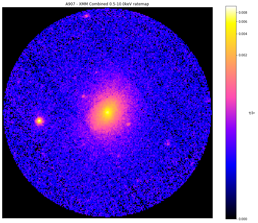
Viewing XGA Photometric products
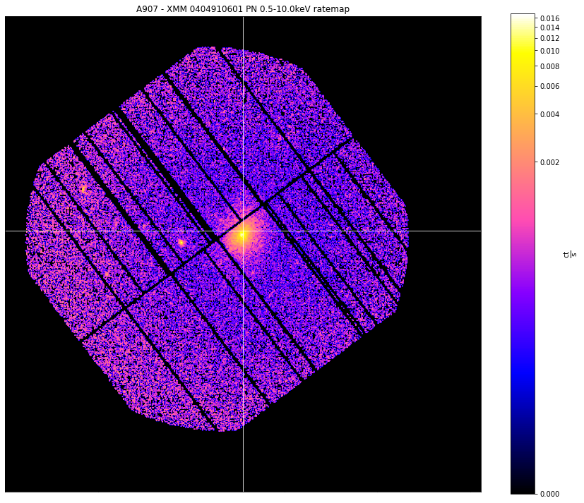
One of the most useful features built into XGA’s photometric products is the ability to easily visualise them with the view() method. There are multiple ways to modify the image produced, this includes changing the size of the image, altering the scaling applied (log-scaling is used by default), applying masks, zooming in specific parts of the image, and adding crosshairs to indicate a coordinate.
Again, we’re using a ratemap taken from Abell 907, and with one simple line of code we can produce a useful visualisation. Here the size of the image is increased so that it looks better in the documentation, and used the crosshairs to highlight the coordinate of the user supplied position. Only one crosshair can be placed on an image, but the coordinate can be in degrees, or pixels (or XMM sky coordinates for XMM images):
[28]:
# Displaying the ratemap, with a crosshair for a particular coordinate
chosen_ratemap.view(cross_hair=demo_src.ra_dec, figsize=(12, 10))
Retrieving a value at a certain coordinate
At some point you may wish to know the value of a photometric product at a certain coordinate, a ratemap or an exposure map for instance. There are built in methods to help you retrieve those values which will accept coordinates in any valid unit (degrees, pixels, or XMM sky for XMM products). The value is returned as an Astropy quantity, with the correct units for the type of product.
We demonstrate a useful feature of ratemap, that it stores links to the image and expmap that were used to create it, so accessing those constituent products is as easy as using the ‘image’ or ‘expmap’ properties of the ratemap:
[29]:
# For a ratemap, we use the method 'get_rate'
print(chosen_ratemap.get_rate(demo_src.ra_dec), '\n')

# If we wished to know the exposure time at that position, we could access the ratemap's
#  expmap and use 'get_exp'
print(chosen_ratemap.expmap.get_exp(demo_src.ra_dec), '\n')
0.0062226445925877135 ct / s

4981.8046875 s
Combined images and exposure maps
As there are generated images for all the ObsIDs and instruments associated with the source, it is possible to bring all that information together by creating a combined image. Most XGA analyses take place on combined products, because that ability to find all relevant data for a particular source is one of XGA’s key strengths. For XMM data this is done through XGA’s interaction with the SAS routine emosaic. (eROSITA photometric products already combine all instruments when they are initally generated)
[ ]:
# For the single source
demo_src = emosaic(demo_src, 'image', lo_en=lo_en, hi_en=hi_en)

# For the sample
demo_smp = emosaic(demo_smp, 'image', lo_en=lo_en, hi_en=hi_en)
Similarly this may be done with exposure maps.
[ ]:
# For the single source
demo_src = emosaic(demo_src, 'expmap', lo_en=lo_en, hi_en=hi_en)

# For the sample
demo_smp = emosaic(demo_smp, 'expmap', lo_en=lo_en, hi_en=hi_en)
XGA will then automatically create a combined ratemap, which may be retrieved as follows:
[ ]:
chosen_comb_rt = demo_src.get_combined_ratemaps(lo_en=lo_en, hi_en=hi_en)
This ratemap is used for the rest of this tutorial to demonstrate XGA’s inbuilt photometric functions.
Retrieving and using masks from a source
It is common practise in photometric analyses to mask out any sources that might bias or interfere with the source that you are investigating, and as such each XGA source object is able to produce masking arrays. These masking arrays are filled with ones and zeros, where any zero elements are to be considered ‘masked’, and masked image/expmap/ratemap data can be calculated by multiplying the image/expmap/ratemap data by the masking array.
XGA is capable of producing several types of mask; interloper masks (where non-relevant sources are masked), source masks (where any part of the product not within a certain source region is masked out), and standard masks (which are a combination of the last two types).
An XGA source can generate masks for any of the ObsIDs associated with it.
Now we make a mask that will remove non-relevant sources, a telescope must be specified when generating a mask:
Note that for XMM observations, if no ObsID information is supplied then XGA will assume that the mask should be generated for a combined photometric product.
[40]:
# This generates a mask that removes interloper sources (any non-relevant source). As we
#  didn't provide an ObsID it is only valid for the combined products
interloper_mask = demo_src.get_interloper_mask('xmm')


# It is very easy to apply the mask to remove any interlopers from the ratemap
chosen_comb_rt.view(cross_hair=demo_src.ra_dec, mask=interloper_mask, figsize=(12, 10))
Its just as easy to produce an interloper mask for a specific ObsID, and though the ratemaps look extremely similar, please note that this is because the three XMM observations associated with this source all have near identical pointing coordinates. That means that the shape of this image is very similar to the 512x512 of the individual images. This may not be the case for other sources, where separate observations added together can result in quite different image shapes.
Here we produce a mask for the Abell 907 ratemap we retrieved earlier:
[42]:
# Much the same process as to generate the mask for the combined ratemap, but we also supply an ObsID
individual_interloper_mask = demo_src.get_interloper_mask(obs_id=chosen_ratemap.obs_id, telescope='xmm')

# It is very easy to apply the mask to remove any interlopers from the ratemap
chosen_ratemap.view(cross_hair=demo_src.ra_dec, mask=individual_interloper_mask, figsize=(12, 10))

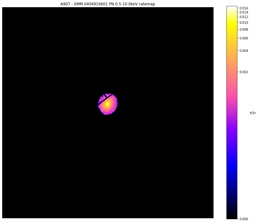
Now we are going to learn how to generate masks that lets us select the source region of interest. At this point we have to make a choice as to which source region we’re interested in; most source objects will allow us to generate a mask from the region files which were supplied to XGA in the configuration file, but if you have a point source then you could also choose ‘point’, and if you have a Galaxy Cluster then you could also select one of the overdensity regions (such as ‘r200’).
When you generate a source region mask, you will also be supplied with a matching background region mask, which is a region extending between back_inn_rad_factor - back_out_rad_factor multiplied by the radius of interest, where these keyword arguments are set when defining a source object.
[45]:
# A source and background mask generated for the selected source from our region file for
# this particular ObsID
region_masks = demo_src.get_source_mask('region', 'xmm', obs_id=chosen_ratemap.obs_id)
# The source mask applied to the 0404910601-PN ratemap in the 0.5-10.0keV range
chosen_ratemap.view(mask=region_masks[0], figsize=(12, 10))
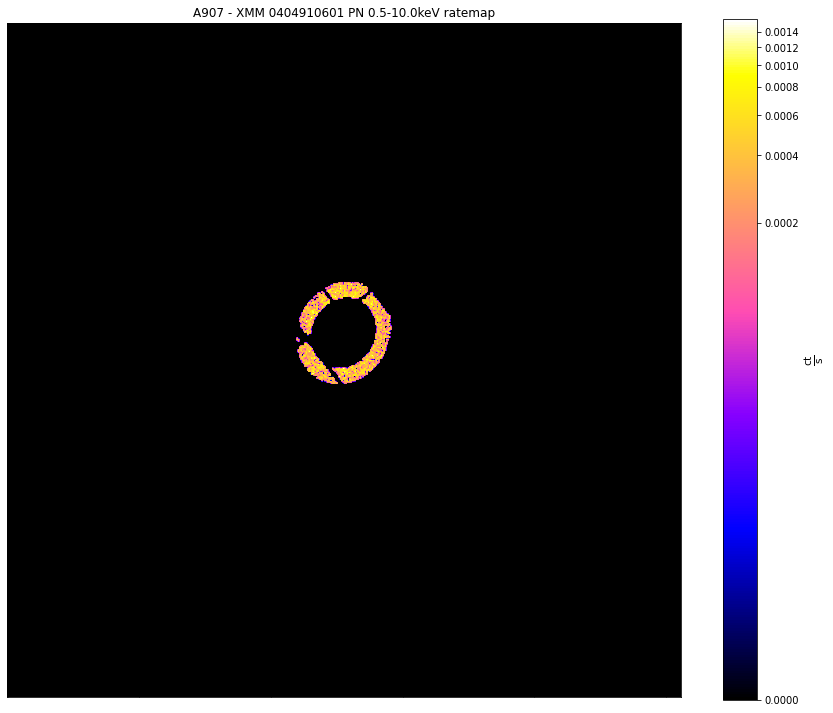
# The show the background mask applied to this ratemap
chosen_ratemap.view(mask=region_masks[1], figsize=(12, 10))
/its/home/jp735/.conda/envs/xga_dev/lib/python3.8/site-packages/ipykernel/ipkernel.py:283: DeprecationWarning: `should_run_async` will not call `transform_cell` automatically in the future. Please pass the result to `transformed_cell` argument and any exception that happen during thetransform in `preprocessing_exc_tuple` in IPython 7.17 and above.
  and should_run_async(code)
/mnt/lustre/projects/astro/general/jp735/XGA_dev/XGA/xga/sources/base.py:3550: UserWarning: You cannot use custom central coordinates with a region from supplied region files
  src_reg, bck_reg = self.source_back_regions(reg_type, telescope, obs_id, central_coord)
/its/home/jp735/.conda/envs/xga_dev/lib/python3.8/site-packages/regions/core/compound.py:93: DeprecationWarning: `np.int` is a deprecated alias for the builtin `int`. To silence this warning, use `int` by itself. Doing this will not modify any behavior and is safe. When replacing `np.int`, you may wish to use e.g. `np.int64` or `np.int32` to specify the precision. If you wish to review your current use, check the release note link for additional information.
Deprecated in NumPy 1.20; for more details and guidance: https://numpy.org/devdocs/release/1.20.0-notes.html#deprecations
  data = self.operator(*np.array(padded_data, dtype=np.int))
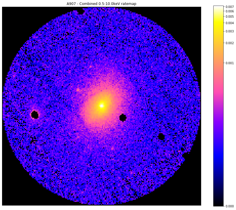
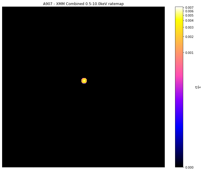
Now we’ve seen how to access a region file region, we’re going to look at an R\(_{500}\) region. We set zoom_in=True which crops around the area with a non-zero value:
[48]:
# A source and background mask generated for the combined ratemap for Abell 907 at R_500
# Note that a telescope must always be parsed to any get_mask method
r500_masks = demo_src.get_source_mask('r500', 'xmm')

# Here I will show the source mask applied to the combined ratemap in the 0.5-10.0keV range
chosen_comb_rt.view(mask=r500_masks[0], figsize=(12, 10), zoom_in=True)
/its/home/jp735/.conda/envs/xga_dev/lib/python3.8/site-packages/ipykernel/ipkernel.py:283: DeprecationWarning: `should_run_async` will not call `transform_cell` automatically in the future. Please pass the result to `transformed_cell` argument and any exception that happen during thetransform in `preprocessing_exc_tuple` in IPython 7.17 and above.
  and should_run_async(code)
/its/home/jp735/.conda/envs/xga_dev/lib/python3.8/site-packages/regions/core/compound.py:93: DeprecationWarning: `np.int` is a deprecated alias for the builtin `int`. To silence this warning, use `int` by itself. Doing this will not modify any behavior and is safe. When replacing `np.int`, you may wish to use e.g. `np.int64` or `np.int32` to specify the precision. If you wish to review your current use, check the release note link for additional information.
Deprecated in NumPy 1.20; for more details and guidance: https://numpy.org/devdocs/release/1.20.0-notes.html#deprecations
  data = self.operator(*np.array(padded_data, dtype=np.int))
Finally, we can still see that there are some obvious point sources remaining in this source region, and for a real analysis we would want to be able to remove them. As such we use the source method ‘get_mask’, and apply it to the same combined ratemap.
It is important to note that the user does not have to generate these masks centered at the default central coordinates for the source object in question, you can also specify another central coordinate using central_coord in a mask generation method.
When we see the image below we can quite clearly see examples of a few point sources that obviously have to be removed before a meaningful analysis of the galaxy cluster can begin:
[23]:
# A source and background mask generated for the combined ratemap for Abell 907 at R_500
r500_interloper_masks = demo_src.get_mask('r500',)

# Here I will show the source mask applied to the combined ratemap in the 0.5-10.0keV range
chosen_comb_rt.view(mask=r500_interloper_masks[0], figsize=(12, 10), zoom_in=True)

Creating a custom mask
A mask may be created with whatever custom radius you desire, custom coordinates to centre the new mask on may be defined, as well as both inner and outer radii (if you wish to make an annulus). In this demonstration a mask with an outer radius of 0.01 degrees is made (though if the source in question has redshift information you can also use a proper distance unit) for the XMM combined image of the demo source:
[50]:
custom_mask = demo_src.get_custom_mask(Quantity(0.01, 'deg'), 'xmm')
custom_mask
[50]:
array([[0., 0., 0., ..., 0., 0., 0.],
       [0., 0., 0., ..., 0., 0., 0.],
       [0., 0., 0., ..., 0., 0., 0.],
       ...,
       [0., 0., 0., ..., 0., 0., 0.],
       [0., 0., 0., ..., 0., 0., 0.],
       [0., 0., 0., ..., 0., 0., 0.]])
[53]:
chosen_comb_rt.view(mask=custom_mask)
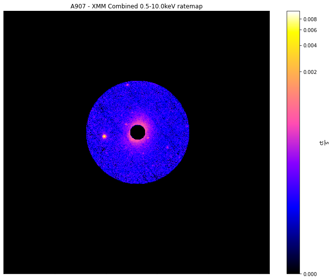
Now we make a mask with the core of this galaxy cluster excised (the mask shall allow everything from 0.15-1R\(_{500}\)), here we set remove_interloper=False, so non-relevant sources remain in the image:
[56]:
custom_mask = demo_src.get_custom_mask(demo_src.r500, 'xmm',
                                       inner_rad=demo_src.r500*0.15,
                                       remove_interlopers=False)
chosen_comb_rt.view(mask=custom_mask)
Measuring signal-to-noise
Measuring the signal to noise of a given source is a fairly common task in astronomy, and an ability which has been implemented and added to the photometric product classes in XGA. It is a simple matter to quickly find the signal to noise of a galaxy cluster within an overdensity radius for instance, you need only call the info() method. There you will find that XGA has automatically measured the signal-to-noise within the supplied overdensity radii:
[57]:
demo_src.info()
-----------------------------------------------------
Source Name - A907
User Coordinates - (149.59209, -11.05972) degrees
---------------------------------------------------------------------------
KeyError                                  Traceback (most recent call last)
Cell In[57], line 1
----> 1 demo_src.info()

File /mnt/lustre/projects/astro/general/jp735/XGA_dev/XGA/xga/sources/base.py:4823, in BaseSource.info(self)
   4821 print("User Coordinates - ({0}, {1}) degrees".format(*self._ra_dec))
   4822 if self._use_peak is not None and self._use_peak:
-> 4823     print("X-ray Peak - ({0}, {1}) degrees".format(*self._peaks["combined"].value))
   4824 print("nH - {}".format(self.nH))
   4825 if self._redshift is not None:

KeyError: 'combined'
If, however, you wish to retrieve the signal to noise programmatically (or measure it within a custom radius), you can simply use the get_snr method. In this demonstration we retrieve the signal to noise of this cluster within the R\(_{500}\) and within a custom radius of 300kpc:
Note that you must parse a telescope argument
[60]:
r500_snr = demo_src.get_snr('r500', 'xmm')
print(r500_snr)
cust_snr = demo_src.get_snr(Quantity(300, 'kpc'), 'xmm')
print(cust_snr)
251.27067538813375
209.05353673494383
/its/home/jp735/.conda/envs/xga_dev/lib/python3.8/site-packages/ipykernel/ipkernel.py:283: DeprecationWarning: `should_run_async` will not call `transform_cell` automatically in the future. Please pass the result to `transformed_cell` argument and any exception that happen during thetransform in `preprocessing_exc_tuple` in IPython 7.17 and above.
  and should_run_async(code)
/its/home/jp735/.conda/envs/xga_dev/lib/python3.8/site-packages/regions/core/compound.py:93: DeprecationWarning: `np.int` is a deprecated alias for the builtin `int`. To silence this warning, use `int` by itself. Doing this will not modify any behavior and is safe. When replacing `np.int`, you may wish to use e.g. `np.int64` or `np.int32` to specify the precision. If you wish to review your current use, check the release note link for additional information.
Deprecated in NumPy 1.20; for more details and guidance: https://numpy.org/devdocs/release/1.20.0-notes.html#deprecations
  data = self.operator(*np.array(padded_data, dtype=np.int))
A simple assessment may be performed determining which observation associated with a given source is ‘the best’, by ranking them by signal to noise of the source. Call the snr_ranking method, supply it with a radius within which to measure the SNR, and it will return an array of ObsID-instrument combinations, and an array of SNR values, going from worst to best:
[63]:
oi_combs, snr_vals = demo_src.snr_ranking('r500')
---------------------------------------------------------------------------
NotAssociatedError                        Traceback (most recent call last)
Cell In[63], line 1
----> 1 oi_combs, snr_vals = demo_src.snr_ranking('r500')

File /mnt/lustre/projects/astro/general/jp735/XGA_dev/XGA/xga/sources/base.py:4737, in BaseSource.snr_ranking(self, outer_radius, lo_en, hi_en, allow_negative)
   4732 for obs_id in self.instruments:
   4733     for inst in self.instruments[obs_id]:
   4734         # Use our handy get_snr method to calculate the SNRs we want, then add that and the
   4735         #  ObsID-inst combo into their respective lists
   4736         snrs.append(
-> 4737             self.get_snr(outer_radius, 'xmm', self.default_coord, lo_en, hi_en, obs_id, inst, allow_negative))
   4738         obs_inst.append([obs_id, inst])
   4740 # Make our storage lists into arrays, easier to work with that way

File /mnt/lustre/projects/astro/general/jp735/XGA_dev/XGA/xga/sources/base.py:3789, in BaseSource.get_snr(self, outer_radius, telescope, central_coord, lo_en, hi_en, obs_id, inst, psf_corr, psf_model, psf_bins, psf_algo, psf_iter, allow_negative, exp_corr)
   3784     rt = self.get_combined_ratemaps(lo_en, hi_en, psf_corr, psf_model, psf_bins, psf_algo, psf_iter,
   3785                                     telescope=telescope)
   3787 elif all([obs_id is not None, inst is not None]):
   3788     # Both ObsID and instrument have been set by the user
-> 3789     rt = self.get_ratemaps(obs_id, inst, lo_en, hi_en, psf_corr, psf_model, psf_bins, psf_algo, psf_iter,
   3790                            telescope=telescope)
   3791 else:
   3792     raise ValueError("If you wish to use a specific ratemap for {s}'s signal to noise calculation, please "
   3793                      " pass both obs_id and inst.".format(s=self.name))

File /mnt/lustre/projects/astro/general/jp735/XGA_dev/XGA/xga/sources/base.py:2796, in BaseSource.get_ratemaps(self, obs_id, inst, lo_en, hi_en, psf_corr, psf_model, psf_bins, psf_algo, psf_iter, telescope)
   2768 def get_ratemaps(self, obs_id: str = None, inst: str = None, lo_en: Quantity = None, hi_en: Quantity = None,
   2769                  psf_corr: bool = False, psf_model: str = "ELLBETA", psf_bins: int = 4, psf_algo: str = "rl",
   2770                  psf_iter: int = 15, telescope: str = None) -> Union[RateMap, List[RateMap]]:
   2771     """
   2772     A method to retrieve XGA RateMap objects. This supports the retrieval of both PSF corrected and non-PSF
   2773     corrected ratemaps, as well as setting the energy limits of the specific ratemap you would like. A
   (...)
   2794     :rtype: Union[RateMap, List[RateMap]]
   2795     """
-> 2796     return self._get_phot_prod("ratemap", obs_id, inst, lo_en, hi_en, psf_corr, psf_model, psf_bins, psf_algo,
   2797                                psf_iter, telescope)

File /mnt/lustre/projects/astro/general/jp735/XGA_dev/XGA/xga/sources/base.py:2031, in BaseSource._get_phot_prod(self, prod_type, obs_id, inst, lo_en, hi_en, psf_corr, psf_model, psf_bins, psf_algo, psf_iter, telescope)
   2027     extra_key = "_" + psf_model + "_" + str(psf_bins) + "_" + psf_algo + str(psf_iter)
   2029 if not psf_corr and with_lims:
   2030     # Simplest case, just calling get_products and passing in our information
-> 2031     matched_prods = self.get_products(prod_type, obs_id, inst, extra_key=energy_key, telescope=telescope)
   2032 elif not psf_corr and not with_lims:
   2033     broad_matches = self.get_products(prod_type, obs_id, inst, telescope=telescope)

File /mnt/lustre/projects/astro/general/jp735/XGA_dev/XGA/xga/sources/base.py:2683, in BaseSource.get_products(self, p_type, obs_id, inst, extra_key, just_obj, telescope)
   2680 # If the telescope IS associated and the ObsID has been supplied then we can check that it is valid
   2681 elif (telescope is not None and telescope in self.telescopes) and \
   2682         (obs_id is not None and obs_id not in self.obs_ids[telescope]):
-> 2683     raise NotAssociatedError("{o} is not associated with the {t} telescope for "
   2684                              "{n}.".format(o=obs_id, n=self.name, t=telescope))
   2685 # Finally we can see if supplied instruments are valid, if telescope and ObsID are supplied
   2686 elif (telescope is not None and telescope in self.telescopes) and \
   2687         (obs_id is not None and obs_id in self.obs_ids[telescope]) and \
   2688         (inst is not None and inst != 'combined' and inst not in self.instruments[telescope][obs_id]):

NotAssociatedError: xmm is not associated with the xmm telescope for A907.
[64]:
oi_combs
---------------------------------------------------------------------------
NameError                                 Traceback (most recent call last)
Cell In[64], line 1
----> 1 oi_combs

NameError: name 'oi_combs' is not defined
[66]:
snr_vals
---------------------------------------------------------------------------
NameError                                 Traceback (most recent call last)
Cell In[66], line 1
----> 1 snr_vals

NameError: name 'snr_vals' is not defined
Bulk generation of photometric products
If you wished to generate images in a particular energy range for a large number of unrelated observations, then you would use a NullSource object.
Normally, when defining a NullSource object, it would automatically associate every available ObsID with itself, but it is possible to pass a list of specific ObsIDs of interest (as done in this demo). These ObsIDs must be parsed as dictionary with telescope top-level keys, if a telescope is not included in this dictionary then every observation will be associated to the NullSource, so here we pass an empty list for eROSITA:
[70]:
# Four randomly select observation that will make up the NullSource
chosen_obs = ['0677630133', '0301900401', '0770581201', '0827201501']
# And defining the source with four unrelated observations associated with it
# This should be parsed as a dictionary with telescope top level keys
bulk_src = NullSource({'xmm': chosen_obs, 'erosita': []})
[71]:
# If we run the standard info() method then we can say a very little information about the source
bulk_src.info()
-----------------------------------------------------
Source Name - AllObservations
User Coordinates - (nan, nan) degrees
nH - nan 1e+22 / cm2

-- XMM --
ObsIDs - 4
PN Observations - 4
MOS1 Observations - 4
MOS2 Observations - 4
With initial detection - 0
Spectra associated - 0
-----------------------------------------------------
/its/home/jp735/.conda/envs/xga_dev/lib/python3.8/site-packages/ipykernel/ipkernel.py:283: DeprecationWarning: `should_run_async` will not call `transform_cell` automatically in the future. Please pass the result to `transformed_cell` argument and any exception that happen during thetransform in `preprocessing_exc_tuple` in IPython 7.17 and above.
  and should_run_async(code)
Now we can generate images for this bulk sample:
[73]:
# And of course we can generate images and exposure maps in the same way as with the other sources
evselect_image(bulk_src, lo_en=lo_en, hi_en=hi_en)
/its/home/jp735/.conda/envs/xga_dev/lib/python3.8/site-packages/ipykernel/ipkernel.py:283: DeprecationWarning: `should_run_async` will not call `transform_cell` automatically in the future. Please pass the result to `transformed_cell` argument and any exception that happen during thetransform in `preprocessing_exc_tuple` in IPython 7.17 and above.
  and should_run_async(code)
[73]:
<xga.sources.base.NullSource at 0x7fb4862a5790>
For NullSources combined photometric products can only be made if the associated observations have a coordinate in common.