Annular Spectra of Extended Sources

This section aims to run through the basics of how to generate, and interact with, annular spectra of extended sources in XGA. This will include running XSPEC fits on the annuli, as you would for a galaxy cluster were you would like to measure a projected temperature profile, and an apec normalisation profile (which was used in gas density profiles tutorial.

I’ll also demonstrate how to use the visualisation abilities which are built in the AnnularSpectra class, how to access results from XSPEC fits for each annulus individually, and how to retrieve annular spectra from where they have been stored in a source object.

from xga.samples import ClusterSample
from xga.sas import spectrum_set
from xga.xspec import single_temp_apec_profile

from astropy.units import Quantity
import numpy as np
import pandas as pd

Yet again we will be using these four clusters from the SDSSRM-XCS sample, the same clusters that were used for the gas density profiles tutorial and the spectroscopy tutorial. There was no particular rationale behind selecting these particular clusters for this demonstration, other than that the observations of them of are a high enough quality that there shouldn’t be any problem generating and fitting the spectra.

# Setting up the column names and numpy array that go into the Pandas dataframe
column_names = ['name', 'ra', 'dec', 'z', 'r500', 'r200', 'richness', 'richness_err']
cluster_data = np.array([['XCSSDSS-124', 0.80057775, -6.0918182, 0.251, 1220.11, 1777.06, 109.55, 4.49],
                         ['XCSSDSS-2789', 0.95553986, 2.068019, 0.11, 1039.14, 1519.79, 38.90, 2.83],
                         ['XCSSDSS-290', 2.7226392, 29.161021, 0.338, 935.58, 1359.37, 105.10, 5.99],
                         ['XCSSDSS-134', 4.9083898, 3.6098177, 0.273, 1157.04, 1684.15, 108.60, 4.79]])

# Possibly I'm overcomplicating this by making it into a dataframe, but it is an excellent data structure,
#  and one that is very commonly used in my own analyses.
sample_df = pd.DataFrame(data=cluster_data, columns=column_names)
sample_df[['ra', 'dec', 'z', 'r500', 'r200', 'richness', 'richness_err']] = \
    sample_df[['ra', 'dec', 'z', 'r500', 'r200', 'richness', 'richness_err']].astype(float)

# Defining the sample of four XCS-SDSS galaxy clusters
demo_smp = ClusterSample(sample_df["ra"].values, sample_df["dec"].values, sample_df["z"].values,
                         sample_df["name"].values, r200=Quantity(sample_df["r200"].values, "kpc"),
                         r500=Quantity(sample_df["r500"].values, 'kpc'), richness=sample_df['richness'].values,
                         richness_err=sample_df['richness_err'].values)

Declaring BaseSource Sample: 100%|██████████| 4/4 [00:01<00:00,  2.08it/s]
Generating products of type(s) ccf: 100%|██████████| 4/4 [00:30<00:00,  7.53s/it]
Generating products of type(s) image: 100%|██████████| 4/4 [00:02<00:00,  1.82it/s]
Generating products of type(s) expmap: 100%|██████████| 4/4 [00:01<00:00,  2.40it/s]
Setting up Galaxy Clusters: 100%|██████████| 4/4 [00:04<00:00,  1.25s/it]

Manually generating sets of annular spectra

There are several functions in XGA designed for generating particular types of profile from a set of annular spectra, and in most cases they will have algorithms designed to automatically decide where they’re going to place annuli. However, it is entirely possible that users will want to decide for themselves where exactly the annuli should be placed, and as such I will initially demonstrate how to manually generate annular spectra for our sample.

The spectrum_set() function is where XGA generated sets of annular spectra by setting up the annular regions (including the removal of interloper sources), running all the SAS commands, and then combining the resulting files into a single AnnularSpectra instance. The full documentation for the function can be found here, but it is quite simple to use, with the most important argument being radii, where you specify what annuli should be generated.

When deciding where the annuli should be placed, please bear in mind that the radii argument expects information on the boundaries of the annuli, so should start at zero if you wish the innermost annulus to be a circle. Here we set up four sets of annuli, one for each cluster:

ann_rads = [np.linspace(0, 1, 5)*demo_smp[0].r500, np.linspace(0, 1.2, 6)*demo_smp[1].r500,
            Quantity([0, 100, 200, 300, 1200], 'kpc'), np.linspace(0, 1, 6)*demo_smp[3].r500]
ann_rads

[<Quantity [   0.    ,  305.0275,  610.055 ,  915.0825, 1220.11  ] kpc>,
 <Quantity [   0.    ,  249.3936,  498.7872,  748.1808,  997.5744,
            1246.968 ] kpc>,
 <Quantity [   0.,  100.,  200.,  300., 1200.] kpc>,
 <Quantity [   0.   ,  231.408,  462.816,  694.224,  925.632, 1157.04 ] kpc>]

These radii were chosen essentially randomly, and have no physical meaning or importance, we merely wish to demonstrate the different ways you might want to define sets of annular boundary radii. Now that we’ve set those up, all we need to do is pass them into the spectrum_set() function, and they will be generated. This function will always generate a spectrum between the first and last entries for each set of radii as well, as it is often convenient to normalise values measured from these spectra by a global value.

The background spectrum defined for the set of annular spectra is generated between back_inn_rad_factor*outermost-radius and back_out_rad_factor*outermost radius - those factors were set when you initially defined the source or sample:

spectrum_set(demo_smp, radii=ann_rads)

Generating products of type(s) spectrum: 100%|██████████| 12/12 [55:25<00:00, 277.13s/it]
Generating products of type(s) annular spectrum set components: 100%|██████████| 54/54 [28:05<00:00, 31.22s/it]

<xga.samples.extended.ClusterSample at 0x7f0851661250>

XSPEC fit to annular spectra

Now we want to fit plasma emission models to the set of spectra (there will be multiple spectra per annulus if there are multiple observations of the source), just as we fit a model to the global spectra we produced in the spectroscopy tutorial. Again we’ll be making use of the XGA XSPEC interface, and the fitting process works in exactly the same way for the constant*tbabs*apec model that describes absorbed plasma emission from a cluster. In this case however, we use the single_temp_apec_profile() function (look here for documentation).

To run a default fit with this model to our set of clusters, we just need to pass the same list of annular boundaries into the fitting function (currently the only model that can be used to fit these profiles):

single_temp_apec_profile(demo_smp, radii=ann_rads)

Running XSPEC Fits: 100%|██████████| 18/18 [00:33<00:00,  1.87s/it]

<xga.samples.extended.ClusterSample at 0x7f0851661250>

If we hadn’t already generated these spectra, this function would actually have run the spectrum_set() function for us, then fit them as we requested, but I wished to demonstrate the use of the annular spectra generation function.

Fetching annular spectra from a source

As is the case for most XGA products, there is a specific method to retrieve annular spectra from a source object, in this case the get_annular_spectra method (you can find the full documentation here). Since we know a priori the radii we used to generate the annular spectra, all we need to do here is to pass those radii and the correct set of annular spectra will be fetched:

cur_ann_spec = demo_smp[0].get_annular_spectra(radii=ann_rads[0])
cur_ann_spec

<xga.products.spec.AnnularSpectra at 0x7f0851650dc0>

Please note that each set of annular spectra is issued a unique ‘set id’ when it is generated, and if you already knew that identifying number you could pass it to the get_annular_spectra() method through the set_id argument and retrieve the correct set of annular spectra.

Visualising annular spectra

Now that we’ve generated, fitted, and retrieved these annular spectra, we might want to visualise the data somehow. Several methods to do just that have been implemented in the AnnularSpectra class.

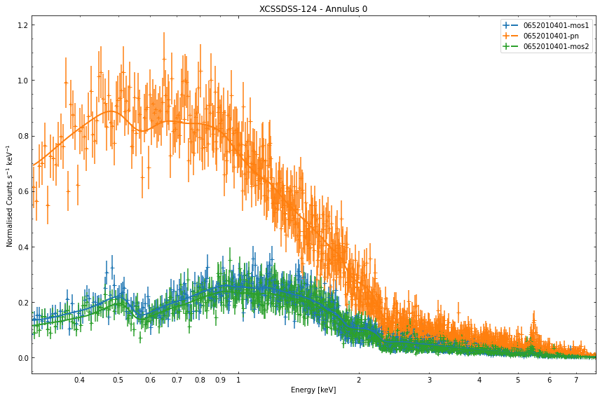
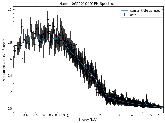
An individual annulus with view_annulus()

The first is akin to the view() method which is present in the Spectrum class, although in this case all spectra for a single annulus are shown. You need to pass the annulus ID (for instance the innermost annulus would be 0, the next 1, etc.), and the model that was fitted (in this case constant*tbabs*apec):

# Just choosing the first annulus for not particular reason
cur_ann_spec.view_annulus(0, 'constant*tbabs*apec')

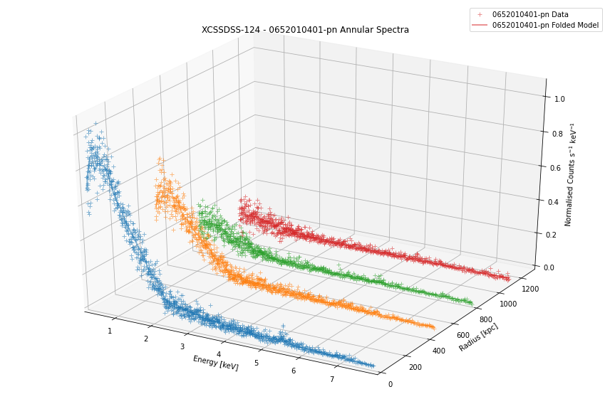
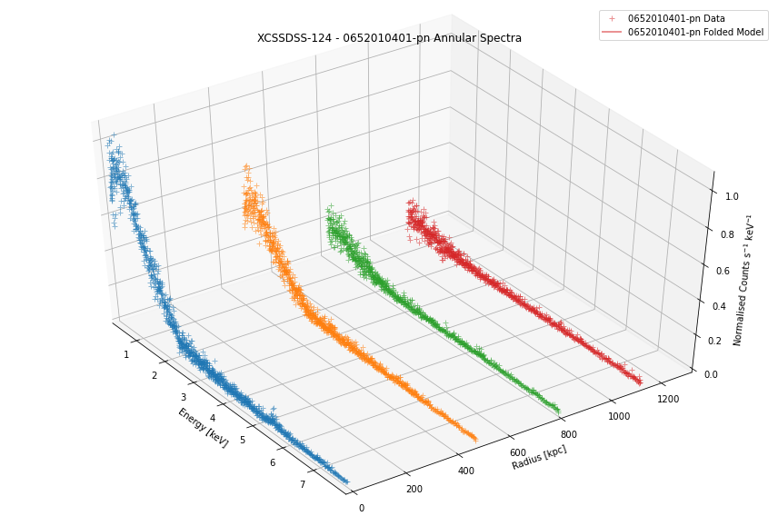
A set of annuli for a particular ObsID-Instrument with view_annuli()

The next method lets you see a whole set of annular spectra, for a single ObsID-Instrument combination. The view_annuli() method requires a little more information, as you have to pass an ObsID and instrument as well as the model that was fitted. This visualisation is in 3D, so you can also set the elevation_angle and azimuthal_angle to change perspective. I also use the instruments property that each source object has to remind myself which ObsIDs and instruments are associated with this source:

demo_smp[0].instruments

{'0652010401': ['pn', 'mos1', 'mos2']}

cur_ann_spec.view_annuli('0652010401', 'pn', 'constant*tbabs*apec')

# Changing the perspective, just a demonstration I'm not saying this is more useful
cur_ann_spec.view_annuli('0652010401', 'pn', 'constant*tbabs*apec', elevation_angle=45, azimuthal_angle=-35)

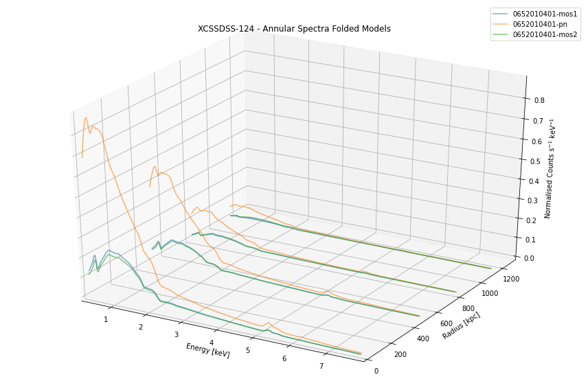
All fitted models for all annuli with view()

Another three dimensional view method, but rather than a set of annular spectra for a specific ObsID-instrument combination, this will show the fitted models for all ObsID-instrument combinations associated with this AnnularSpectra instance. No data points are plotted here because it makes the figure far too confusing. The same angle arguments can be passed to change the perspective of the plot:

cur_ann_spec.view('constant*tbabs*apec')

Retrieving a spectrum from an AnnularSpectra instance

An AnnularSpectra instance is what is termed an ‘aggregate product’ in XGA; that is to say that its actually a container for multiple individual product instances (in this case Spectrum instances). That means that those individual instances (with all their built in features and information) are stored within the aggregate product, and can be retrieved with a convenient get method (get_spectra() in this case).

So if we decided we wanted to retrieve the 0652010401-pn spectrum for the innermost annulus, we would run this command:

ind_spec = cur_ann_spec.get_spectra(0, '0652010401', 'pn')

Then we could decide to view that spectrum, if we wanted:

ind_spec.view()

We aren’t limited to retrieving one spectrum at a time however, if we wanted to we could grab a list of all the Spectrum objects that make up the first annulus:

cur_ann_spec.get_spectra(0)

[<xga.products.spec.Spectrum at 0x7f08568e8ca0>,
 <xga.products.spec.Spectrum at 0x7f08568e8e20>,
 <xga.products.spec.Spectrum at 0x7f08568e8880>]

If, for some reason, you wanted to do the same thing but for all spectra in the AnnularSpectra object, you could just use the all_spectra property:

cur_ann_spec.all_spectra

[<xga.products.spec.Spectrum at 0x7f08568e8ca0>,
 <xga.products.spec.Spectrum at 0x7f08568e8e20>,
 <xga.products.spec.Spectrum at 0x7f08568e8880>,
 <xga.products.spec.Spectrum at 0x7f08568e8850>,
 <xga.products.spec.Spectrum at 0x7f08568e8760>,
 <xga.products.spec.Spectrum at 0x7f08568c7580>,
 <xga.products.spec.Spectrum at 0x7f08568e8be0>,
 <xga.products.spec.Spectrum at 0x7f08568e8340>,
 <xga.products.spec.Spectrum at 0x7f085690d0a0>,
 <xga.products.spec.Spectrum at 0x7f08568c5040>,
 <xga.products.spec.Spectrum at 0x7f085690dd60>,
 <xga.products.spec.Spectrum at 0x7f08568e8220>]

Retrieving fit results and luminosities

Retrieving fit results is as simple as calling another get method, get_results. You must specify which annulus you want to get the results for, as well as the model that was fitted, and optionally you can specify the name of the parameter that you particularly want to grab:

cur_ann_spec.get_results(0, 'constant*tbabs*apec')

{'kT': array([7.41271   , 0.12935868, 0.1301684 ]),
 'norm': array([4.2421700e-03, 3.3772432e-05, 3.4043752e-05]),
 'factor': array([[0.958273  , 0.00932076, 0.00942246],
        [1.0042    , 0.01143088, 0.01155637]])}

cur_ann_spec.get_results(3, 'constant*tbabs*apec', 'norm')

array([3.66600000e-04, 2.16666992e-05, 2.19063438e-05])

The behaviour of the method with which you fetch luminosities (get_luminosities) is much the same, but instead of optionally specifying a parameter name you can pass lo_en and hi_en values to get back a luminosity measured within specific energy limits:

cur_ann_spec.get_luminosities(0, 'constant*tbabs*apec')

{'bound_0.5-2.0': <Quantity [2.95390183e+44, 1.75799566e+42, 1.42047898e+42] erg / s>,
 'bound_0.01-100.0': <Quantity [1.16941378e+45, 1.26719656e+43, 1.23961762e+43] erg / s>}

cur_ann_spec.get_luminosities(0, 'constant*tbabs*apec', lo_en=Quantity(0.5, 'keV'), hi_en=Quantity(2.0, 'keV'))

$[2.9539018 \times 10^{44},~1.7579957 \times 10^{42},~1.420479 \times 10^{42}] \; \mathrm{\frac{erg}{s}}$

Other useful information about AnnularSpectra

Here I will quickly run through other useful pieces of information which are stored in an AnnularSpectra object. The first piece of information that can be handy is the number of annuli in a given spectrum, for which you can just use the standard Python len() function (or the num_annuli property):

print(len(cur_ann_spec))
print(cur_ann_spec.num_annuli)

4
4

There is also a property that will return the set id that, as I mentioned earlier, is a unique identifier that can be used to retrieve the AnnularSpectra object:

cur_ann_spec.set_ident

1295248

The boundary radii which were used to generated the set of annular spectra initially are given by the radii property:

cur_ann_spec.radii

$[0,~0.020943087,~0.041886174,~0.062829261,~0.083772348] \; \mathrm{{}^{\circ}}$

And finally, the obs_ids property gives a list of all the ObsIDs that went into the AnnularSpectra (it is essentially the same as the obs_ids property of BaseSource), and AnnularSpectra has an instruments property that performs the same function as the instruments property of BaseSource:

cur_ann_spec.obs_ids

['0652010401']

cur_ann_spec.instruments

{'0652010401': ['mos1', 'pn', 'mos2']}