Basics of XGA profiles - focusing on cluster surface brightness
Here the aim is to go through the basic capabilities of XGA profile products, with a focus on the generation of surface brightness profiles of galaxy clusters. A demonstration of the fitting functionality built into XGA profiles will be given, which will include an exploration of the XGA model classes and their purpose. I’ll also show how we can view profiles (both for individually and together), and run through the user-configurable options built into the view method.
Given the nature of this analysis, it isn’t really applicable to point-like sources.
[1]:
from xga.sources import GalaxyCluster

from astropy.units import Quantity
import numpy as np
Firstly, I will define a GalaxyCluster source for Abell 907, a cluster for which I know high quality data is available. Again, please note that the overdensity radius and redshift that I’ve used here are approximate and should not be used for a scientific analysis:
[2]:
src = GalaxyCluster(149.59209, -11.05972, 0.16, r500=Quantity(1200, 'kpc'), name='A907')
src.info()
-----------------------------------------------------
Source Name - A907
User Coordinates - (149.59209, -11.05972) degrees
X-ray Peak - (149.59251340970866, -11.063958320861634) degrees
nH - 0.0534 1e+22 / cm2
Redshift - 0.16
XMM ObsIDs - 3
PN Observations - 3
MOS1 Observations - 3
MOS2 Observations - 3
On-Axis - 3
With regions - 3
Total regions - 69
Obs with one match - 3
Obs with >1 matches - 0
Images associated - 18
Exposure maps associated - 18
Combined Ratemaps associated - 1
Spectra associated - 0
R500 - 1200.0 kpc
R500 SNR - 251.61
-----------------------------------------------------
Generating and viewing a surface brightness profile
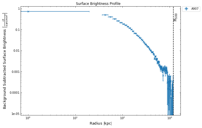
A convenient method for quickly generating and viewing cluster surface brightness profiles has been implemented in the GalaxyCluster source class, with the main input being the desired outer radius of the brightness profile in question. In this demonstration I have made a profile out to the approximate R\(_{500}\) that I supplied on declaration, and by default this method has used the combined brightness profile to do so:
[3]:
src.view_brightness_profile('r500')
The view_brightness_profile method doesn’t actually create the brightness profile itself however, it is simply a wrapper around the radial_brightness function implemented in the ‘imagetools’ section of XGA. I will not go into detail on how the generation is undertaken, but the end result is an instance of the XGA SurfaceBrightness1D class. I will
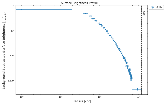
mention, however, that you can supply minimum quality requirements when generating these profiles, for instance requiring each bin to have a minimum signal to noise, as shown here:
[4]:
src.view_brightness_profile('r500', min_snr=1.1)
Retrieving the SurfaceBrightness1D instance from the source
It is likely that you want to do more than just look at the profile, so the next step is to extract it from wherever it has been stored in the source object. Most profile types have a specific get method, but a general get_profiles method also exists, which I shall show first. We have to supply the profile type, with a ‘combined_’ prefix to indicate that the profile was generated using combined data:
[5]:
src.get_profiles('combined_brightness')
[5]:
[<xga.products.profile.SurfaceBrightness1D at 0x7fa2fdbb7520>,
 <xga.products.profile.SurfaceBrightness1D at 0x7fa32c685b50>]
We can see that because we only supplied the type of profile we want, both the brightness profiles we generated have been returned to us. If we specifically wanted the profile we generated out to \(R_{500}\) without any automatic re-binning however, we can use the get_1d_brightness_profile method and tell it that the outer radius of the profile we want is R\(_{500}\) (something that, after the re-binning applied to the second profile, is no longer true for both):
[6]:
sb_prof = src.get_1d_brightness_profile('r500')
sb_prof
[6]:
<xga.products.profile.SurfaceBrightness1D at 0x7fa2fdbb7520>
Saving XGA profiles to disk
All profiles generated by XGA are automatically saved to the {xga save path}/profiles/{source name} directory, so that if the same source is declared again at some point in the future then they can be loaded back in without having to run the generation again. Running the generation procedure again for brightness profiles wouldn’t be much of a problem, considering how fast it is, but other profiles take considerably more time to generate.
A profile will generally automatically re-save itself when a change (such as fitting a model) is made to it, and you can manually save it by calling the save() method and passing a path.
The profile is saved by pickling the profile instance, which can result in some relatively large files if there are many points and model fits stored within the profile:
[7]:
sb_prof.save("random_brightness_profile.xga")
If you have a profile object loaded in then you can access the automatic save path which XGA has assigned it by using the save_path property:
[8]:
sb_prof.save_path
[8]:
'/home/dt237/code/PycharmProjects/XGA/docs/source/notebooks/advanced_tutorials/xga_output/profiles/A907/brightness_profile_A907_58634018.xga'
Fitting a model to the SurfaceBrightness1D instance
So, we’ve generated this profile, and now we’ve decided we want to be able to represent it with a model. You, as a new user, don’t know a priori what models have been implemented for whatever profile type you’re working with; as such you should call the allowed_models() method, which will tell you what models you’re allowed to fit:
[9]:
# Passing grid here changes the style of the table. The default style looks nicer in my opinion, but LaTeX
#  has a hard time rendering it for the PDF version of this documentation
sb_prof.allowed_models('grid')
+--------------+---------------------------------------------+-----------------------------------------+
| MODEL NAME   | EXPECTED PARAMETERS                         | DEFAULT START VALUES                    |
+==============+=============================================+=========================================+
| beta         | beta, r_core, norm                          | 1.0, 100.0 kpc, 1.0 ct / (arcmin2 s)    |
+--------------+---------------------------------------------+-----------------------------------------+
| double_beta  | beta_one, r_core_one, norm_one, beta_two,   | 1.0, 100.0 kpc, 1.0 ct / (arcmin2 s),   |
|              | r_core_two, norm_two                        | 0.5, 400.0 kpc, 0.5 ct / (arcmin2 s)    |
+--------------+---------------------------------------------+-----------------------------------------+
Now that you can see which models you’re allowed to fit to this particular type of profile, we might decide that we’re going to fit the simple beta model. There are a couple of slightly different ways we could decide to do this, with the simplest being we just pass the name of the model as a string to the fit method of the profile. This would declare an instance of that model class, with the default starting values and priors, and then fit it.
Alternatively, we could decide that we want to customise the model parameters, declare an instance of that particular model manually, and pass it to the fitting function. I’m going to demonstrate this approach, so I can introduce you to the way models work in XGA; firstly, we have to import the model that we chose:
[10]:
# I do not condone importing anywhere but the top of a Jupyter notebook, but it
#  helps the demonstration to do it here
from xga.models import BetaProfile1D
When we called the allowed_models method we were shown the default start values for the model parameters, including the required units, and so we can declare suitable astropy quantities now as we declare a new model instance with non-standard start values (the model will error if start parameters with the wrong units are passed):
[11]:
beta_inst = BetaProfile1D(cust_start_pars=[Quantity(0.8), Quantity(50, 'kpc'), Quantity(0.6, 'ct/(arcmin^2 s)')])
beta_inst.start_pars
[11]:
[<Quantity 0.8>, <Quantity 50. kpc>, <Quantity 0.6 ct / (arcmin2 s)>]
I am not claiming that these are ‘better’ start values than the default ones for this particular cluster, I am simply doing this for demonstrative purposes. Model classes have many built in methods, some of which provide visualisations of the model, some provide convenient access to derivatives and integrated values, and some just provide general information about the model:
[12]:
beta_inst.info('grid')
+-----------------+-----------------------------------------------------------------------------+
| Beta Profile    |                                                                             |
+=================+=============================================================================+
| DESCRIBES       | Surface Brightness                                                          |
+-----------------+-----------------------------------------------------------------------------+
| UNIT            | ct / (arcmin2 s)                                                            |
+-----------------+-----------------------------------------------------------------------------+
| PARAMETERS      | beta, r_core, norm                                                          |
+-----------------+-----------------------------------------------------------------------------+
| PARAMETER UNITS | , kpc, ct / (arcmin2 s)                                                     |
+-----------------+-----------------------------------------------------------------------------+
| AUTHOR          | placeholder                                                                 |
+-----------------+-----------------------------------------------------------------------------+
| YEAR            | placeholder                                                                 |
+-----------------+-----------------------------------------------------------------------------+
| PAPER           | placeholder                                                                 |
+-----------------+-----------------------------------------------------------------------------+
| INFO            | Essentially a projected isothermal king profile, it can be                  |
|                 | used to describe a simple galaxy cluster radial surface brightness profile. |
+-----------------+-----------------------------------------------------------------------------+
We can also see and alter the default priors that have been set for the model parameters. Though this is largely only relevant if you wish to fit with the MCMC option, and at the moment is limited to uniform priors. The par_priors property returns the priors in the form of a list of dictionaries:
[13]:
beta_inst.par_priors
[13]:
[{'prior': <Quantity [0., 3.]>, 'type': 'uniform'},
 {'prior': <Quantity [   0., 2000.] kpc>, 'type': 'uniform'},
 {'prior': <Quantity [0., 3.] ct / (arcmin2 s)>, 'type': 'uniform'}]
The par_priors property is also how you set new priors, by passing another list of dictionaries in the same format (an error will be thrown if there aren’t the correct number of priors, or if the units are incorrect):
[14]:
beta_inst.par_priors = [{'prior': Quantity([-1., 4.]), 'type': 'uniform'},
                        {'prior': Quantity([   1., 1400.], 'kpc'), 'type': 'uniform'},
                        {'prior': Quantity([0., 2.], "ct / (arcmin2 s)"), 'type': 'uniform'}]
beta_inst.par_priors
[14]:
[{'prior': <Quantity [-1.,  4.]>, 'type': 'uniform'},
 {'prior': <Quantity [1.0e+00, 1.4e+03] kpc>, 'type': 'uniform'},
 {'prior': <Quantity [0., 2.] ct / (arcmin2 s)>, 'type': 'uniform'}]
Now that we’ve setup our model instance, we’re going to fit it to the profile. There are several fitting methods implemented in the profile base class, including one based on the emcee ensemble MCMC sampler, one based around scipy’s ‘curve_fit’ implementation of non-linear least squares, and one based around scipy’s implementation of orthogonal distance regression. We shall use the MCMC fitter here, with a simple gaussian likelihood, as I wish to demonstrate some of the extra
features that are enabled with an MCMC fit. I will mention again that you could just pass ‘beta’ as the first argument here if you just wished to use the default beta model setup:
[15]:
sb_prof.fit(beta_inst, num_steps=30000, num_walkers=20)
100%|██████████| 30000/30000 [00:33<00:00, 905.55it/s]
[15]:
<xga.models.sb.BetaProfile1D at 0x7fa2fdce7ca0>
The fit method will return a model instance (in this case the same one we passed in), which has had the fit results added to it, though you can also retrieve the fit directly from the profile object (as the model is stored internally). We have to specify the name of the model as well as the fit type, as the same type of model can be fitted and stored with multiple fit methods:
[16]:
sb_prof.get_model_fit('beta', 'mcmc')
[16]:
<xga.models.sb.BetaProfile1D at 0x7fa2fdce7ca0>
Exploring the fitted model
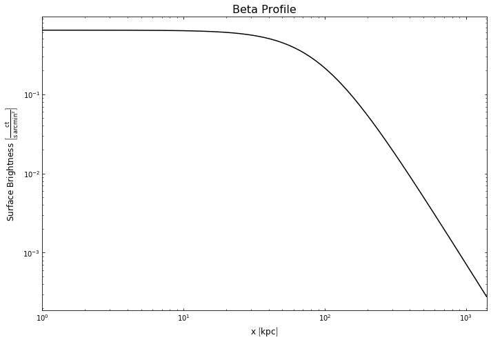
Due to the fact that we setup our own model instance prior to running the fit method (and the way Python memory addressing works), we can actually just look at our initial beta_inst model, we don’t need to retrieve it from the object or the fit method (notice we never assigned their return to a variable). The model class has three visualisation methods implemented, though they are meant more for convenience than for the production of publishable figures. We can view the model curve (if we
pass radii at which we wish to calculate values), and the parameter distributions from the fit:
[17]:
# We have to pass radii at which to evaluate the model, I just pass a set of radii
#  from 1 (because its a log scale by default) to 1400kpc.
beta_inst.view(Quantity(np.arange(1, 1400, 1), 'kpc'), figsize=(10,7))
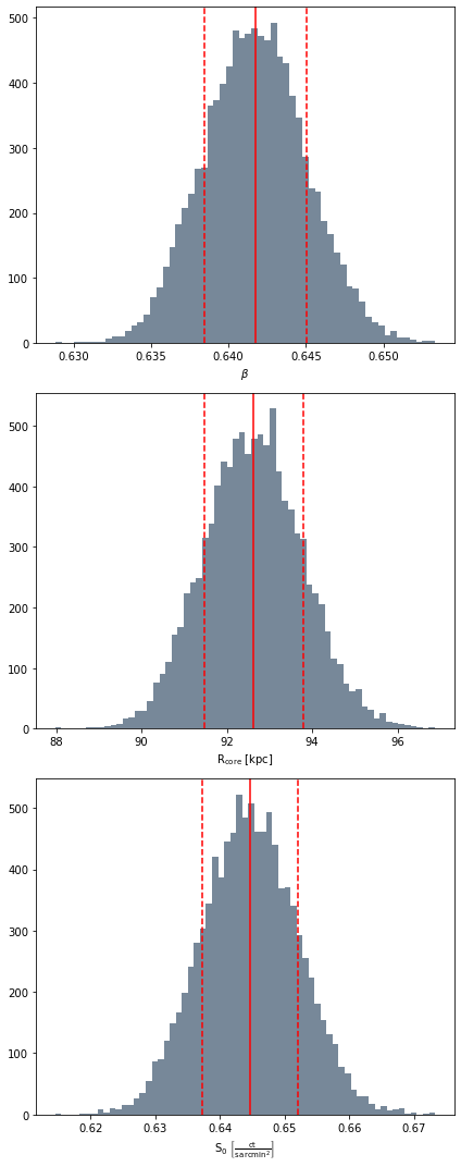
[18]:
beta_inst.par_dist_view()
Mathematics with the fitted model
There are various ways of interacting with the model mathematically, the simplest of which is using the fitted model to predict a value at a particular radius. For this you just need to call the model instance and pass the radius at which you wish to evaluate the model, no further information is required as the knowledge of the model parameter values is stored within the instance:
[19]:
beta_inst(Quantity(600, 'kpc'))
[19]:
By default this returns a single value, using the best fit values to predict it; however more often than not a single value is not very useful, we need knowledge of the uncertainty associated with it. In this case we can use the parameter posterior distributions to calculate a value distribution at the given radius:
[20]:
beta_inst(Quantity(600, 'kpc'), use_par_dist=True)
[20]:
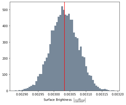
On a slight side note, you can also have a quick look at the predicted distribution in histogram form:
[21]:
beta_inst.predicted_dist_view(Quantity(600, 'kpc'))
If you have a model instance and wanted to make a prediction using parameter values other than those from the fitting process, you can use the model method and manually pass parameters:
[22]:
beta_inst.model(Quantity(600, 'kpc'), Quantity(2, ''), Quantity(240, 'kpc'), Quantity(2, 'ct/(arcmin^2s)'))
[22]:
There are also convenient ways to calculate derivatives of the model, and again we can either return a single value or a distribution (again by setting the use_par_dist argument). In general, if there is an analytical solution to the 1st derivative of a model that has been implemented in XGA, then the analytical solution is what is being used to calculate the value. If there is no analytical solution then the scipy derivative function is being used, and the user must pass an appropriate
dx value - this function is also what is used to calculate nth order derivatives:
[23]:
beta_inst.derivative(Quantity(600, 'kpc'))
[23]:
[24]:
beta_inst.nth_derivative(Quantity(600, 'kpc'), dx=Quantity(0.01, 'kpc'), order=2, use_par_dist=True)
[24]:
Other mathematical functions include inverse_abel for performing inverse abel transforms on the models, and volume_integral, for performing volume integrals using the model. You can read more about them in the BaseModel1D API documentation.
Back to the profile
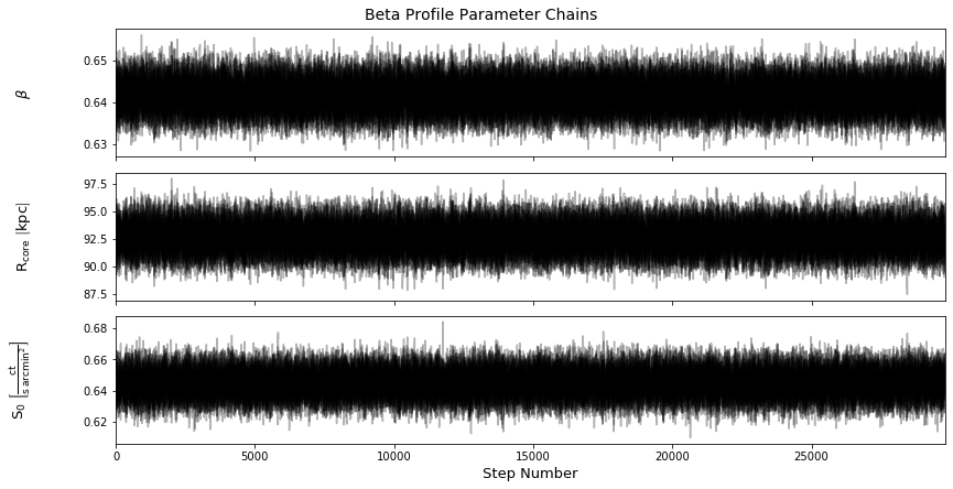
Now that I’ve shown you a bit of what you can do with the actual model object, I’m going to show you how the surface brightness profile object we started with makes use of the model. Firstly we can take a look at the MCMC chains produced during the fitting of the model using the view_chains() method, and again we must tell the method what the name of the model is:
[25]:
sb_prof.view_chains('beta')
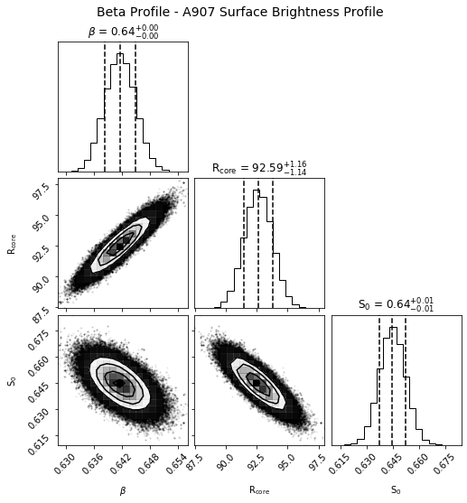
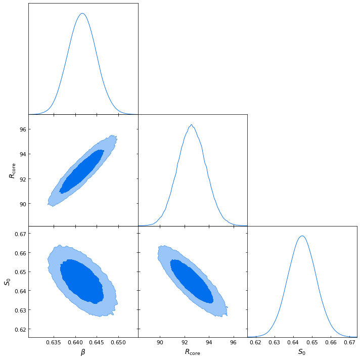
We can also make the contour plots which are so often seen in relation to MCMC, both using the corner module and the getdist module, depending which you prefer:
[26]:
sb_prof.view_corner('beta')
[27]:
sb_prof.view_getdist_corner('beta')
Removed no burn in
WARNING:root:fine_bins_2D not large enough for optimal density
WARNING:root:fine_bins_2D not large enough for optimal density
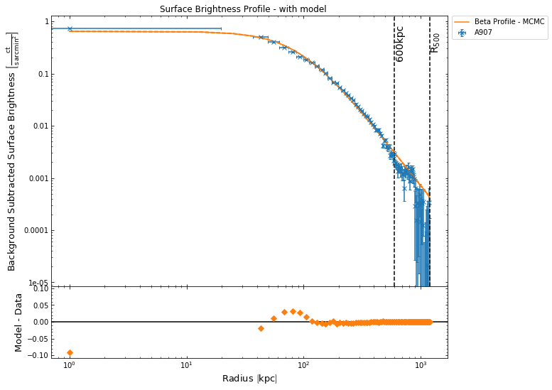
We can now view the profile with both data and model shown, using the profile view() method, and add some lines indicating particular radii using the draw_rads argument. There are a few other ways that users can configure the plots generated by the profile view() method, and they can be explored in the method documentation:
[28]:
sb_prof.view(draw_rads={'600kpc': Quantity(600, 'kpc'), 'R$_{500}$': src.r500})
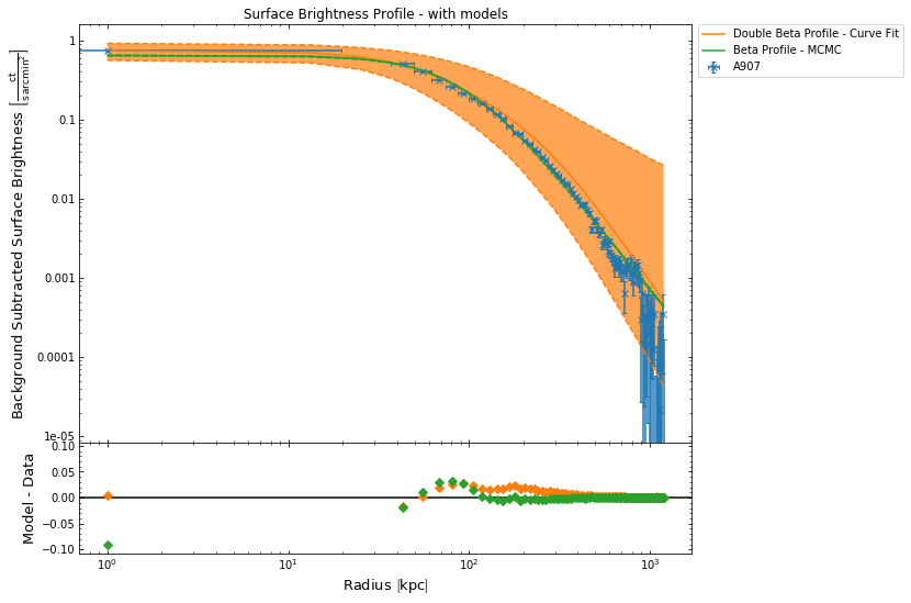
If we were to fit another model to this profile, and then view the profile, it would also be included in the plot generated by this view() method. To demonstrate this I will quickly fit a default double beta model to the profile (this time with the curve fit method), and then view the profile once again:
[29]:
sb_prof.fit('double_beta', method='curve_fit')
sb_prof.view()
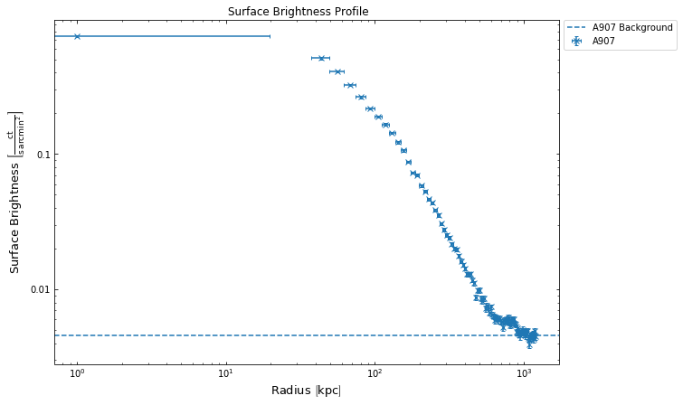
We can also turn off the plotting of the models entirely, as well as the background subtraction:
[30]:
sb_prof.view(models=False, back_sub=False)
Viewing multiple profiles on one plot
It is often the case that we wish to view multiple profiles on a single plot, either for a comparison or to present results from a sample of objects. This is very easy to do with XGA profiles due to the introduction of the BaseAggregateProfile1D class, an instance of which contains multiple profile objects and allows them to easily be plotted together. The simplest way to create such an object is to add two (or more) profiles together, just using the normal ‘+’ Python operator, though be aware that an error will be thrown if the profiles are not all of the same type.
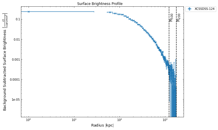
To demonstrate this I will declare another galaxy cluster object, and view the surface brightness profile to make sure one is generated:
[31]:
other_src = GalaxyCluster(0.80057775, -6.0918182, 0.251, 'XCSSDSS-124', r500=Quantity(1220.11, 'kpc'),
                          r200=Quantity(1777.06, 'kpc'))
other_src.view_brightness_profile('r200')
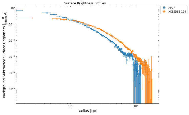
Then I will simply add the profile I just created for XCSSDSS-124 to the profile we have been using throughout this tutorial, then call the view() method, just as I did before:
[32]:
(sb_prof + other_src.get_1d_brightness_profile('r200')).view()